Normal Distribution

The normal distribution curve is also referred to as the Gaussian Distribution (Gaussian Curve) or bell-shaped curve. Manufacturing processes and natural occurrences frequently create this type of distribution, a unimodal bell curve.

A normal distribution exhibits the following:

68.3% of the population is contained within 1 standard deviation from the mean.

95.4% of the population is contained within 2 standard deviations from the mean.

99.7% of the population is contained within 3 standard deviations from the mean.

The distribution is spread symmetrically around the central location which happens when occurrences are equally above and below an average.

Mean = Mode = Mean

Skewness = 0

Kurtosis = 3

Coefficient of Variation = standard deviation / mean

A visual depiction of the standard deviation of normal distribution

Normal Distribution at Six-Sigma-Material.com

These three figures should be committed to memory if you are a Six Sigma GB/BB.

These three figures are often referred to as the Empirical Rule or the 68-95-99.5 Rule as approximate representations population data within 1,2, and 3 standard deviations from the mean of a normal distribution. in the above picture, the mean is assumed = 0.

Over time, upon making numerous calculations of the cumulative density function and z-scores, with these three approximations in mind, you will be able to quickly estimate populations and percentages of area that should be under a curve.

Most Six Sigma projects will involve analyzing normal sets of data or assuming normality. Many natural occurring events and processes with "common cause" variation exhibit a normal distribution (when it does not this is another way to help identify "special cause").

This distribution is frequently used to estimate the proportion of the process that will perform within specification limits or a specification limit (NOT control limits - recall that specification limits and control limits are different).

However, when the data does not meet the assumptions of normality the data will require a transformation to provide an accurate capability analysis.

Normal Distribution Quiz

If a normal distribution has a mean of 75 and a standard deviation of 10, 95% of the distribution can be found between which two values?

A) 0, 95

B) 65, 85

C) 55, 95

D) 45, 105

Answer: C. 95% of the distribution (area under the curve) is 1.96 standard deviations from the mean which can be estimated at 2. Therefore 75-20 = 55 is the lower value and 75+20 = 95 is the upper value.

If a normal distribution has a mean of 35 and a variance of 25, 68% of the distribution can be found between which two values?

A) 30, 40

B) 25, 45

C) 0, 70

D) 20, 50

Answer: A. 68% of the distribution (area under the curve) is about +/- 1 standard deviation from the mean. The standard deviation is the square root of the variance and therefore = 5. Therefore 35-5 = 30 is the lower value and 35+5 = 40 is the upper value.

A normally distributed population has a mean of 5 km, standard deviation of 0.2 km, variance of 0.04 km, what is the median?

A) 5 km

B) 1 km

C) 0.2 km

D) None of the above

Answer: A. In a normal distribution, the mean = median = mode.

A distribution of measurements for the length of widgets was found to have a mean of 92.0mm and a standard deviation of 2.50mm. Approximately what percent of measurements are between 87.00mm and 97.00mm?

A) 100%

B) 68%

C) 95%

D) 99%

Answer: C. The measurements of 87.00mm and 97.00mm are two standard deviations away from the mean of 92.00mm. Therefore about 95% of the values recorded are between 87.00mm and 97.00mm.

The mean is used to define the central location in a normal data set and the median, mode, and mean are near equal. The area under the curve equals all of the observations or measurements.

Throughout this site the following assumptions apply unless otherwise specified:

P-Value < alpha risk set at 0.05 indicates a non-normal distribution although normality assumptions may apply. The level of confidence assumed throughout is 95%.

P-Value > alpha risk set at 0.05 indicates a normal distribution.

The z-statistic can be derived from any variable point of interest (X) with the mean and standard deviation. The z-statistic can be referenced to a table that will estimate a proportion of the population that applies to the point of interest.

Recall, one of two important implications of the Central Limit Theorem is, regardless distribution type (unimodal, bi-modal, skewed, symmetric), the distribution of the sample means will take the shape of a normal distribution as the sample size increases. The greater the sample size the more normality can be assumed.

Some tables and software programs compute the z-statistic differently but will all get the correct results if interpreted correctly.

Some tables incorporate single-tail probability and another table may incorporate double-tail probability. Examine each table carefully to make the correct conclusion.

The bell curve theoretically spreads from negative infinity to positive infinity and approaches the x-axis without ever touching it, in other words it is asymptotic to the x-axis.

The area under the curve represents the probabilities and the whole area is estimated to be equal to 1.0 or 100%.

The normal distribution is described by the mean and the standard deviation. The formula for the probability density function (PDF) of the normal distribution is:

Density function for normal distribution

Due to the time-consuming calculations using integral calculus to come up with the area under the normal curve from the formula above most of the time it is easier to reference tables.

With pre-populated values based on a given value for "x", the probabilities can be assessed using a conversion formula (shown below) from the z-distribution, also known as the standardized normal curve.

The z-distribution is a also called the standard normal distribution with:

Mean = 0
Standard Deviation = 1

A z-score is the number of standard deviations that a given value "x" is above or below the mean of the normal distribution.

Any normal distribution can be standardized by converting its values into z-scores. A z-score is many standard deviations from the mean a value lies.

Example

A machining process has produced widgets with a mean length of 12.5 mm and variance of 0.0625 mm.

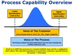
A customer has indicated that the upper specification limit (USL) is 12.65 mm. What proportion of the bars will be shorter than 12.65 mm.

Process Mean: 12.5 mm
Process Standard Deviation = 0.25 mm (square root of 0.0625)
Point of Interest (x): 12.65 mm
The z-score = (12.65 - 12.5) / 0.25 = 0.60

From the table below which is a one-tailed table it shows that 0.60 corresponds to 0.7257.

72.57% of the area under the curve is represented below the point of x = 12.65 mm.

The means that 72.57% of the widgets will be below the USL of the customer. This result will not likely meet the Voice of the Customer.

Using Excel in the example above

Use the formula:

NORM.DIST (x, mean, standard deviation, True)

True uses the Cumulative Density Function (CDF) and False uses the Probability Density Function (PDF).

ADDITIONAL INSIGHT:

If the standard deviation of the process was tighter (lower), such as 0.05mm then that indicates the process is more predictable and consistent than before and the spread of the process performance is narrower around the mean.

Therefore, more parts would be expected to be bunched up around the process mean. Substituting, 0.05mm in place of 0.25mm, gives the 99.865%.

Does that make sense?

A process with mean 12.5 mm and standard deviation of only 0.05 mm AND the USL is 12.65 mm. You would expect that almost 100% should of the parts should be under the USL of 12.65 mm......and that is the result 99.865%.

=NORM.DIST(12.65,12.5,0.05,TRUE)

use the table for z-score of 3.0 = 0.9987 = 99.87% (see the table below).

In summary, the process still has the same mean of 12.5mm but this time it is more precise and therefore can achieve the customer specification almost 100% of the time.

Is that good enough?

It sounds excellent...relative to the previous result and it is significantly better than before; however, this still may not be acceptable to the customer. As a GB/BB, you'll need to obtain the Voice of the Customer and determine is their acceptable defect rate.

If the customer demands <0.1% defectives, then the process mean needs to shift lower and/or the standard deviation must get lower yet.

Parametric and Non Parametric Tests

Once the data is determined to take on a normal distribution (or assumed to be normal) it indicates that the center value for the distribution of data is the mean.

For nonparametric test the measure of central tendency for the distribution of data is the median.

Parametric tests are generally more powerful assuming the same amount of data that nonparametric test for ANOVA and t-test. It is easier (fewer samples) to determine a significant difference) using parametric tests.

Whenever possible (without forcing or skewing data) a GB/BB should try to satisfy the assumptions of normality. The tests are generally easier to apply and work through from a statistical perspective. Most of certification programs will focus more on the parametric tests.

Click here to access hypothesis test flowcharts for choosing the proper test to use for various parametric and non-parametric data.

Normal Distribution Table
(Members get access to a free download with several tables. Click here to learn more)

Assumption of Normality

We have an entire module dedicated to hypothesis testing of data to determine whether it can be assumed to be from a normal distribution. We also cover the various tests and applications of the normal distribution in a Six Sigma project.

Click here to open the webpage regarding the assumption of normality.

Non-Normal Data

When the data set is not normally distributed, the Central Limit Theorem usually applies or a transformation of the data, such as a Box-Cox or Johnson transformation applies. This determination MUST be done prior to using hypothesis testing tools.

There are cases when the data distribution will naturally not adhere to a normal distribution. Such as the:

time to respond to a customer
time to deliver a product to a customer
annual income of all employees within a large manufacturing company

In the first two cases, naturally there will be a lower bound (can not get lower) of 0 seconds but there will not be an upper bound. The data will not likely center around an average but most of the results will be toward the left side, toward 0 seconds and the tail will have those fewer instances that each took a long time.

In the last case, most employees will make within a certain range and then there will be directors, vice-presidents, and executives that gross higher incomes.

The likely output will look similar to the histogram below, a right-skewed distribution:

Right Skewed Distribution

There are various functions used to transform data such as logarithm, power, square root, and reciprocal. Two of the most common are:

Box-Cox Transformation
Johnson Transformation

Use the help menu in the statistical software package to guide you in transforming data and it is also a good idea to consult with your mentor to ensure it is being done necessarily and correctly.

Using the reciprocal method is straightforward. Apply the equation y = 1/x. Each data point value becomes its reciprocal. If the original data points (x) were 5, 8, 10, 4, 6, then the transformed data (y) becomes 1/5, 1/8, 1/10, 1/4, and 1/6 respectively.

The Box-Cox transformation uses a power transformation but is limited to positive data.

Return to BASIC STATISTICS

Return to DMAIC

Templates and Calculators

Subscribe for complete access to Six-Sigma-Material.com

Return to the Six-Sigma-Material Home Page

ShareFacebook X WhatsApp