Z-score
(sigma score or standardized score)

Description:

The z-score calculation can be done a couple of ways. This score used in the MEASURE as a baseline measurement and in CONTROL phase (for a final score) of a DMAIC Six Sigma project.

The formula below converts a point of interest (x) in terms of standard deviations from the population mean. This is the value to be "standardized".

It allows the comparison of observations from different normal distributions. If the value of x is less than the mean, then the z-score is negative and vice versa. Other names for the z-score are z-values, normal scores, and standardized score.

Calculating z-score from a normal set of data

Z-scores at Six-Sigma-Material.com

Objective:

Determine a baseline z-score in the MEASURE phase after the MSA has passed. This preliminary value provided in the project contract may need refinement, this exercise is done in the MEASURE phase to get an accurate starting point.

Another z-score is calculated in the CONTROL phase. Sometimes it is done at the end of the IMPROVE phase but either way it is the final score indicating the change (better or worse) relative to the baseline measurement.

The z-score is most often used in the z-test in the Student's t-test for a population whose parameters are actually known (not estimates). But since it is rare to know the entire population, the t-test is more commonly used.

Z Score Calculator

Another way to calculate z-score

Depending in the information provided, you may not know the inputs for the formula above and instead you may have to use DPU, DPO, DMPO, and Yield to get the sigma score.

For example:

If you had 100 orders delivered and 11 of them were late and another 5 were incorrect, calculate the z-score.

Let's break this down step by step.

Total Defects: 16 (11 + 5 which is the sum the late orders + incorrect orders)

# of Units: 100 orders

# of Defect Opportunities per Unit: 2 (late & incorrect)

DPU: 16/100 = 0.16 (or 16%)

DPO: 16/(100*2) = 0.08 (8%)

DPMO: 0.08 *1,000,000 = 80,000

Throughput Yield (TPY) = 1 - DPO = 1 - 0.08 = 0.92 (TPY is 92%)

Sigma Level (using Excel): norm.s.inv(%Yield) + 1.5 = norm.s.inv(0.92) + 1.5σ

= 1.405σ + 1.5σ = 2.905σ

OR find TPY (using formula shown later)

TPY = e^(-DPO) = 2.71828^(-0.08) = 0.92 = 92%

NOTE:

The 1.5σ is the assumed shift for short term performance which is the theoretical best-case scenario or entitlement.

The important part of the calculation is to get the DPO value. Once you have that then the Yield is easy to calculate which is 1 - DPO.

In this case, your team is starting with baseline measurement of 80,000 DPMO (or 1.405 sigma) and the goal is to get to 3.4 DPMO (which is 4.5 sigma long term but Six Sigma performance in the short term).

See how it works:

3.4 DPMO = 0.0000034 DPO.

And the Yield = 1 - DPO which is 1 - 0.0000034 = 0.9999966

Using Excel, norm.sin.v(0.9999966) = 4.5 sigma and then add 1.5 sigma (for short term performance) and that equals 6σ!

So 3.4 DPMO = 4.5 sigma (LT) which is 6.0 sigma (ST)

Z-bench (a.k.a. Z-benchmark)

A benchmark sigma (z-bench) score offers a fair comparison for products or processes. A benchmark z-score is often unknown at the onset of the Project Contract and is a critical component for a GB/BB to determine as early as possible in the DMAIC project path.

Once the baseline is determined then the contract is updated and all key stakeholders and revisit the potential savings and impact of the project and possibly redefine the scope.

The GB/BB's job is to collect the necessary data once the MSA passes to calculate and convert this data to a sigma score.

A couple simple useful formulas as estimates (if the DPO is small) are:

TPY = e^(-DPO)
Sigma (z) = NORM.S.INV(TPY) using Excel

If your data represents a shorter time frame or a short-term sample then it is important to consider applying the 1.5 sigma shift to indicate what the longer-term performance would actually be as a baseline. Further below is an explanation on converting short term to long term z-scores.

Recall e is the exponential constant and is approximately 2.71828

Virtual learning videos

Intro Stats: Using a Z-Score Table (2 of 2) from Teacher 2 Open High School on Vimeo.

Using TI Calculators to find z-score

Click here to be redirected to a presentation that shows how to calculate z-scores on TI graphing calculators.

Short Term versus Long Term

Explaining the 1.5 sigma shift

Motorola is credited with concluding that processes drift over long periods of time. The term is known as Long-Term Dynamic Mean Variation or in simpler terms, the "fudge factor". This variation between the short-term samples was determined to be approximately 1.5 sigma.

Long term indicators contain both special cause and common cause variation. Short term data does not contain special cause variation and usually has a higher process capability than the long-term data. That implies that the z-score for a short-term sample should usually be higher than the z-score from long term data.

Six Sigma projects usually report process capability in terms of short-term performance. The true long-term performance is estimated to have some special cause and unexpected performance (since Motorola confirmed this after years or study) and therefore estimated to be 1.5 sigma lower than the short-term z-score.

It is possible to estimate the long or short-term performance based on that value. A GB/BB can apply the 1.5 sigma shift if converting to or from long term sigma or short-term sigma (if you are a believer in this 1.5 sigma shift).

If the z-score was calculated from a sample then the long-term performance can be estimated by subtracting 1.5 sigma from your calculated value for short term sigma.

Recall that if you arrive at DPMO that is considered a long term process indicator but it may not be if you have populations normally in the billions or trillions. It is important to use the shift appropriately. Using enough process data a GB/BB can even estimate the shift for their own process.

If the value you came up with was from a population it is a long term representation of the process performance. Therefore, if interested in the projected short-term performance then you would add 1.5 from your calculated z-score.

Going LONG TERM ---> SHORT TERM: + 1.5 SIGMA

Going SHORT TERM ---> LONG TERM: - 1.5 SIGMA

If the point of interest (x) is located on the mean then the z-score is zero. This seems logical since the point lies directly on the mean with zero standard deviation from the mean.

If the point of interest (original measurement, x) is below the mean then the z-score will be negative. The z-score is positive when the x is a value higher or to the right of the mean.

Z-Distribution

This distribution is represented by a normal distribution with a mean of 0 and a standard deviation of 1. Since integral calculus is challenging to most of us, there are tables to help solve z-distribution and normal distribution problems. Click here for normal distribution table.

The empirical rule for a normal distribution says that about 99.73% of all x values are within 3 standard deviations of the mean which, in terms of a z-distribution, is represented by z = -3 to z = +3.

Converting Z-scores

When a population is normally distributed, the percentile rank may be determined from the z-score and statistical tables. It is important to understand the table being used as websites or textbooks display the values in different ways.

This is most often the most challenging part to a newer GB/BB and common mistake made on exams and projects. Get comfortable with converting z-scores to percentile ranks, PPM's, DPMO, and using tables.

Example One

Data was collected on the production rate of 30 production runs of one part number. The data shows an average of 102 parts per minute with a standard deviation of 10. Calculate the z-score on one of the runs that ran at 142 parts per minute.

The p-value of the 30 runs was <0.05 so we are going to assume normality in this case.

A) 40

B) 4.0

C) 10

Answer B. The point of interest, x, = 142. Therefore z = (142-102) / 10 = 4.

If using Excel, the formula looks like this

Example Two

Given a normally distributed set of data we know the following:

The mean is known to be 52.0
The standard deviation is 4.5

Our point of interest (x) is 61.0

Since the point of interest is greater than the mean you can expect a positive z-value. Substituting the values into the formula at the top of the page:

z = (61 - 52) / 4.5 = 2

The value of 61 is 2 standard deviations (2σ) away from the mean.

Using Excel: =STANDARDIZE (61,52,4.5)

LET'S REVIEW:

Using the assumptions of a normal distributed bell curve only: Take a look at the standardized normal distribution below.

Substitute 52 where the 0 is (the mean) and 61 would go where the 2 is shown. The area greater than 61 (or 2 using the picture below is ~2.5% and the area less than 61 is the other 97.5% of the curve.

~2.5% of the samples are expected to be >61
~97.5% will be under the point of interest of 61.

Using Excel to get the Cumulative Distribution Function (CDF) under the point of interest 'x".

= NORM.DIST(61,52,4.5,TRUE) = 0.97725 (which is same as our estimated ~97.5%)

Normal Distribution with sigma scores on the x-axis

Example Three

Given a normally distributed set of data we know the following:

The mean length is 510.7 mm
The standard deviation of the lengths is 1.49 mm

The customer specifies that the LSL is 507 mm and the USL is 513 mm.

What is the total % of parts that can be expected to be defective?

This is a two-part problem.

FIRST: Determine the % of parts >513 mm.

z = (513 mm - 510.7 mm) / 1.49 mm = 1.54

Referring to a z-table that score equates to 6.8%

SECOND: Determine the % of parts <507 mm.

z = (507 mm - 510.7 mm) / 1.49 mm = -2.48

Referring to a z-table that score equates to 0.66%

The total expected defective parts related to the length are:

6.8% + 0.66% = 7.46%

Example Four

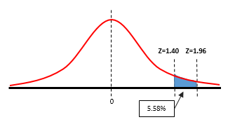
What is the probability that z is <= to 1.96 and >= 1.40?

This is a two step problem since you are looking for an area within the standard random normal distribution curve. Using the table below

P(1.96) = 0.9750

Think of this as representing 97.5% of the total area under the entire bell curve. See the table below to see how the 0.9750 was found.

Next,

P(1.4) = 0.9192 consider 91.92% of the total area under the entire bell curve. See the table below to see how the 0.9192 was found.

Finding z-scores at Six-Sigma-Material.com

The area of interest is found by taking the total area under P(1.96) and subtracting the area under P(1.40). In other words, take 97.5% of the area and subtract 91.92% of the area and the remaining is the area of interest.

P(1.40 <= Z <= 1.96) = 0.9750 - 0.9192 = 0.0558

5.58% of the total area is under the entire standard normal distribution curve is in this region. This is the probability that z is within the region.

Reminder:

Be careful on the table being used. The above table is a two tailed table. A one-tailed table would show P(1.96) = 0.4750 and P(1.40) = 0.4192. The difference in the two values also equals 0.0558.

0.4750 represents the area from the peak of the bell curve (x=0) to the point of z=1.96 which is 47.5% of half the bell curve.

Also, the answer would be the same if the question asked for the P(-1.96 <= Z <= -1.40). This is simply the same area (probability) but on the other side of the bell curve.

Example Five

A Six Sigma Black Belt has compiled the following information regarding computer chips for a DMAIC project and wants to determine the baseline sigma score in the MEASURE phase.