Histograms

Components of a Histogram (Frequency Chart)

Each vertical bar represents an interval of data or a category of data
The x-axis represents the measurements
The y-axis is the frequency
All bars are adjacent and will not overlap since they represent a certain interval (group) of measurements at a specified frequency.

The histogram, when made up of normally distributed data, will form a "bell" curve when a smooth probability density function is produced using kernel smoothing techniques. This line that generalizes the histogram appears to look like a bell.

Often the more data being analyzed and with more resolution will create more bars since more intervals or categories of data are available to plot. The more measurements at various frequencies will create more bars and fill up more of the area under the probability density function.

To assess the data there should be at least 5 bars or intervals and at least 30 data points.

There are a variety of histograms with some explained below. This is also a useful visual tool to depict the skewness and kurtosis of a distribution.

Left-Skewed Distribution (Negatively Skewed):

These histograms have the curve on the right side or the most common values on the right side of the distribution. The data extends much farther out to the left side. These distributions are common where there is an upper specification limit (USL) or it is not possible to exceed an upper value, also known as a boundary limit.

This may occur if a customer has requested the process run at towards the upper specification limit as opposed to targeting the mean.

The measure of central location is the median.

Mean < Median < Mode

Left Skewed Distribution

Right Skewed Distribution (Positively Skewed):

The distribution of the data reaches far out to the right side. This may be caused by a process having a lower boundary. Cost or time plots commonly exhibit this behavior.

The measure of central location is the median.

Mode < Median < Mean

If most common value is 10, the middle most value is 15, and the average of the data set is 20, then the distribution is right skewed.

Mode = 10
Median = 15
Mean = 20

NOTE:

When testing a data set such as this (or left-skewed), for normality, it is like to have a p-value = 0. This means it is very likely the data are not from a normal distribution. You can transform the data, such as using a log transform. If the transformed p-value is >0.05 (or your chosen alpha-risk) then proceed with a parametric test. You cannot do this for bi-modal data. These data must be separated and analyzed separately.

The plotting of Salaries is an example that typically follows a right-skewed distribution since most salaries are centered on a the median but there is a long tail to the "right" that represents the few much higher salaries.

Right Skewed Distribution

Bi-modal Distribution:

These histograms appear to have two or more (polymodal) behaviors occurring in one process and appear to have two points of central location. This can be caused by two sets of data being analyzed as one that are from different populations such as plotting the heights of females and males as one distribution.

Bi-modal Distribution

Uniform Distribution:

The distribution is flat or not exhibiting much of a bell shape and has no appearance of a central location. This may occur when all values between a lower specification limit (LSL) and upper specification limit (USL) are weighted equally acceptable. In other words, values very close to the limits are as a good as a value in the middle.

Click here for more information on the Uniform Distribution.

Uniform Distribution

Normal Distribution:

Points are evenly distributed among a central value or location.

The mean is used to describe the central location of distribution. The median, mode, and mean are all close to the same value AND the Coefficient of Skewness is close to zero.

Click here for more information on the Normal Distribution.

Normal Distribution at Six-Sigma-Material.com

Cumulative Histogram

The plots below depict a regular and a cumulative histogram of the same data. The data shown is 10,000 points randomly sampled from a normal distribution with mean of 0 and standard deviation of 1. The x-axis labels are represent the z-scores.

Notice the cumulative histogram gradually increases to 10,000 (to represent all the data points) and the ordinary histogram shows that data points as they fall into certain data intervals.

Coefficient of Skewness

Karl Pearson is credited with developing the formula below to measure the Coefficient of Skewness. The formula compares the median with the standard deviation of the same distribution.

If:

Sk > 0 then skewed right distribution
Sk = 0 then normal distribution
Sk < 0 then skewed left distribution

Creating a Histogram in Minitab

See the screenshots below (newer versions may show different menus). Go to GRAPH > HISTOGRAM.

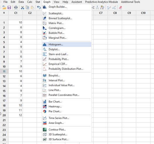
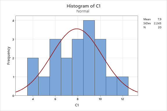
Upon selecting 'Histogram' there are a bunch of options and selections to choose if you wish. In the example below, we choose the date in C1 and select 'OK'.

Notice the very basic information is shown where the mean is 7.9 with a standard deviation of 2.245 among the 20 samples.

Going a step further. Let's assess normality. It appears to be normal based on the eye test but go to STAT > BASIC STATISTICS > GRAPHICAL SUMMARY to dive further.

Enter 'C1' in the Variables box and choose a Confidence Level (default is 95.0%) which represents an alpha-risk of 0.05.

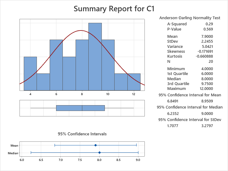
Draw your attention to the P-value which is 0.569. This is much higher than the alpha-risk chosen of 0.05 so the data can be assumed normal. Notice the mean and median are very close which is another good sign to assume normality

For good measure, if it is practical and possible, gather 10 more samples for a total of 30 and rerun these steps.

Some distributions will not meet the assumption of normality; they don't occur naturally as normal distributions. Don't try to force it. Sometimes outliers are legitimate as well and they are part of the process.

To run a hypothesis test, you may need to transform the data or use a non-parametric test.

Other Histogram Examples

Minitab has an option to lay histograms over one another which is just another quick visual tool to help you understand what is happening within the data.

An empirical cumulative distribution, aka empirical cumulative distribution function, of the same data above is shown below by gender.

This cumulative distribution function (CDF) is a step function (look closely and notice the blue lines in each chart) that jumps up by 1/n at each of the n data points. Its value at any specified value of the measured variable is the fraction of observations of the measured variable that are less than or equal to the specified value.

The empirical distribution function is an estimate of the CDF that generated the points in the sample.