|

 content.")
ANOVA
Analysis of Variance
ANOVA is used to determine if there are differences in the mean in groups of continuous data. It answers the question...Is the mean of at least one group different than the mean of other (multiple) groups of data?
The test is used in the ANALYZE phase of a DMAIC project. A GB/BB should be very comfortable understanding the mechanics behind this test. It's likely to be one of the most common tests you will use as a Six Sigma project manager.
ANOVA is commonly used as a hypothesis test for means (not median or mode) applied for testing >2 means (use 1-sample t or 2-sample t test for one or two means respectively).
This module will focus one 1 FACTOR ANOVA. It is possible to have 2, 3, 4, and more factors but most the most common for Six Sigma users is 1-WAY (1 FACTOR) ANOVA.
Assumptions
- Each sample is normally distributed.
- Each sample has equal variances.
- Each sample is independent. There are no patterns or trends present. The changing of one data point should not change another.
- The Y-data is variable type of data (such as time).
- The X-data is attribute data (such as appraiser name).
One Way ANOVA Applications
- Determine if the injury rate among a few manufacturing facilities is different
- Determine if salaries are different among those with various types of degrees
- Determine if salaries vary among institution for the same degree
- Determine if there is a difference among machine production rates for same part
- Determine if a type of treatment works differently on a patient
- Determine if various foods have impact on cholesterol level
- Determine crop output when applying various fertilizers
- Determine if fuel efficiency is different among various driving surfaces
As you read some of the hypothesis, you may tell yourself that there are clearly other factors that could be involved. Hence, the reason for 2, 3 Factor ANOVA's.
A One-Way ANOVA provides some information but ensure to bump that up against other possibilities, common sense, and reality.
Components
ANOVA uses two components of variance and the F test to test the two components:
- BETWEEN sample variance
- WITHIN sample variance
BETWEEN sample variance is a study of the variation among all the samples usually due to process difference or factor changes.
WITHIN
sample variance explains the variation within each sample itself (look
at a Box Plot of one data set to graphically comprehend this - the tip
of one whisker to another).
ANOVA answers the question if the
means of several populations are statistically different or equal. It
also computes a lot of other valuable insight that can help steer a
GB/BB in a clearer direction. A statistical difference is found when the
difference BETWEEN samples is large enough "relative to the difference
WITHIN the samples.
The t-test are limited to comparing up to just two groups. Whereas, ANOVA can compare 3 groups, 15 groups, 25 groups, and more. Using ANOVA to compare two sample means is equivalent to using a t-test to compare the means of independent samples.
ANOVA Jargon
Factor (Process Input Variable - PIV, x): A controlled or
uncontrolled variable (independent variable) whose influence is being
evaluated.
Factor Level (+1,-1, Hi, Low, + , - , A, B): Factor setting.
Response (Process Output Variable - POV, y): The output of the process.
Inference Space: Range of the factors being evaluated.
Fit: Predicted value of the POV (y) with a specified setting of factors.
Residual: Difference from the fit and actual experimental output.
Hypothesis Testing
The following illustrates how the hypothesis test is written along with comments:
HO: Mean 1 = Mean 2 = Mean 3 = Mean n
where n = number of samples or levels or samples
HA: at least 1 Mean is different from the other Means
(read that carefully....it is possible that only one sample mean is different from the other 3, 50, or 100 sample means. Removing the one sample could completely change the result of the test. That is why visual depiction, such as Box Plots, can help find the drivers to the test result or samples that are flawed).
If the Null Hypothesis, Ho, is found to be true, then we would not expect
to see a lot of variation Between Samples. All the population means are considered equal.
If Ho is not true, expect to see significant variation between the samples. This would imply that the difference between samples is large relative to the variation within samples.
Reminder: Statistical significance does not always imply practical significance. Every numerical result needs to be taken under scrutiny to determine if it makes sense in reality.
Follow these steps for One-Way ANOVA:
- State the Practical Problem
- Determine the Factor and Levels of Interest
- Determine the alpha risk (typically 5%)
- Determine the beta risk (typically 10-20%)
- Establish the Effect Size (Epsilon E)
- Establish the Sample Size and collect samples
- Plot the data visually (such as a Box Plot)
- Construct the ANOVA table
- Calculate the test statistic (F) and p-value
- Run the ANOVA hypothesis test for equal means*
- Verify assumptions are met (normality) and examine the residuals
- If the Ho was rejected, determine which mean(s) are different. Looking at the Box Plot and Confidence Intervals are easy way to pick them out. Fisher's Pair-Wise comparison is another statistical method.
- Calculate Epsilon-squared. This explains the % of variation from a given factor. A low value may indicate that other factors may exist.
- Review statistical conclusion and state the practical conclusion. State the level(s) that are different if such is determined.
* If the p-value is less than a, reject Ho and infer HA. If the p-value is greater than alpha risk, fail to reject the Ho

One-Way ANOVA Example
In a completely randomized design (One-way ANOVA) there is only one independent variable (factor or "x") with >2 treatment levels (you could also use this for two levels) also called classifications. The sample sizes do not have to be equal.
Determine
if there is a significant difference of means in two or more appraisers.
The results of a mock study where four appraisers were timed to make an
inspection decision on 13 widgets.
All other criteria are equal.
Since
TIME is the only factor, this is a One-Factor or One-Way ANOVA. There
are four levels that are controlled in the experiment, one being each
appraiser.
The first step is to create the test. In general, if
the p-value is lower than the alpha-risk then the alternate hypothesis
is inferred (reject the null).
Hypothesis Test:
Null Hypothesis: Population means of the different appraisers are equal.
Alternate Hypothesis: One of the means are not the same
There are 51 Degrees of Freedom computed from (13*4) - 1.
Using a One-Way test with an alpha-risk of 0.05, the p-value is well above 0.05 at 0.847 (see results table below).
The F-statistic, and heavily overlapping confidence intervals are also evidence that there is no difference among any pairs or combinations of them.
It is concluded that there is not a statistical difference between any of the appraisers.
What if?
If the p-value was <0.05, then at least one group of data is different than at least one other group. It doesn't conclude which one...only states that at least one of the four is different than the others.

Other notes:
Paul has the lowest average time per appraisal but Jim has lowest variation and the most consistent time for each appraisal. What this result doesn’t say is if the appraisals are correct!
With these results a Six Sigma Project Manager would likely be very pleased that all are performing the same in terms of time spent making an appraisal and the variation from appraisal to appraisal is similar among each person (hopefully the correct appraisal too).
This is likely a result of consistent training and adherence to the SOP's. However, the next questions from the Six Sigma Project Manager is....can this be improved or is it acceptable?
Caution: It still may be possible that 19-20 seconds per appraisal is not acceptable by the company, or customer, and this still needs to be reduced. This One-Way ANOVA only indicates that there is not a statistical difference among the appraisers times. This test is not comparing the appraisers to a target value.
ANOVA results also help understand Variation
The low F-statistic of 0.27 says the variation within the appraisers is greater than the variation between them.
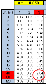
The F-critical value is 2.81 according to the statistical software (not shown above).
You can use the F-table above to get a close estimate of the F-critical value. One downfall with tables is sometimes you may not get a precise number since not every combination is shown. However, the table can provide a fairly good estimate and at least allow a decision to be very conclusive.
The numerator has 3 degrees of freedom and the denominator has 48 degrees of freedom. Using the table below shows that the F-critical value is going to be between 2.76 and 2.84.
And in this case, both values are much higher than the F-calculated value of 0.27 so the conclusion is the same.
As a Six Sigma project manager it may be worth re-running (depending on cost and time) the trial with a larger sample size and additional appraiser training to reduce the variation within each one.
The variation is fairly consistent among each of them so it appears there is a systemic issue that is causing nearly similar amounts of variation within each appraiser.
It is possible that one, or a few, of the widgets are creating a similar spread in the timing for each appraiser. You may want to examine the timing performance of each widget and run an ANOVA among the 13 widgets and see if one or more stands out.
Epsilon-squared is the % of variation related to the Factor, which is the Appraiser. This is 4.84 / 291.69 = 0.01659 = 1.7%. This is a low value so it is possible that other Factors exist that are creating the variation.
ANOVA - Example Two in Excel
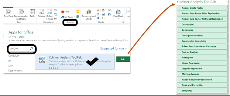
Depending on the version of Excel there is an “Analysis ToolPak” add-in module that may be needed. In this version depicted below it is called "XLMiner Analysis ToolPak". Go to the INSERT tab in this case (or could be under TOOLS).
Type in ANOVA and click on the magnifying glass, the the XLMiner option will appear. Select ADD and the menu will pop up as shown on the right of the picture below.
As you can see, there are several statistical tool to choose from. In this case, select ANOVA: Single Factor
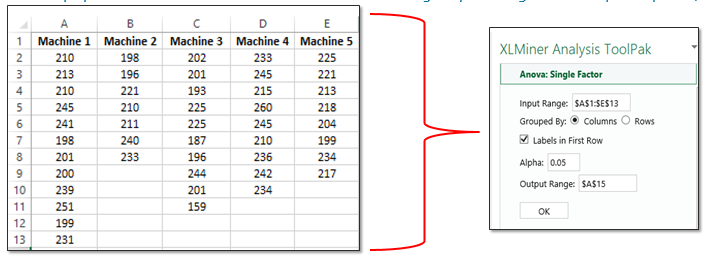
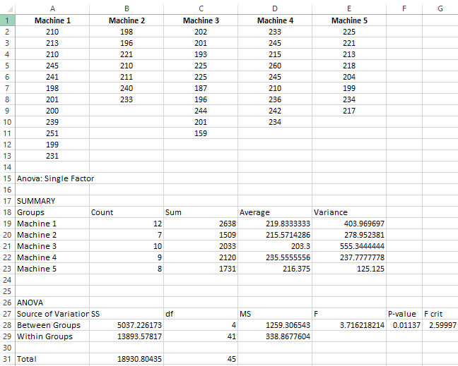
The following data was recorded across five machines. The team recorded the pieces per minute that were produced of the same PN 123XYZ under similar operating conditions and had to be acceptable pieces.
They want to examine several things with one of them being if any of the machines mean performance varied from the other. Assume 95% Confidence Level (0.05 alpha-risk).
For example, the first time that Machine 1 ran a batch of PN 123XYZ it averaged 210 acceptable pieces/minute. Recall, that sample sizes do not have to be the same.
Interpreting the results

Another 1-Way ANOVA result
Let's discuss the following results.

This shows the Set-Up time (hours) of 6 part numbers (levels) on one machine. Assume a 95% Confidence Level which is an alpha-risk of 0.05 (5%)
1) How many samples were analyzed in total? A total of 12+11+15+12+18+16 = 84 samples were studied in this hypothesis test. You don't need the same number of samples for each level (where as a paired t-test you do).
2) What does the p-value tell you? A p-value of 0.019 says that at least one of the level (part numbers) has a different mean than the others. It's pretty clear that PN 13656702 is standing out with the highest mean set-up time of 3.25 hours. Therefore, reject the hull hypothesis (HO) and infer the alternative (HA) which says that at least one mean is different.
3) Which Part Number is playing a big role in lowering the p-value? If you were to remove the data from PN 13656702, the p-value may be >0.05 and thus none of the means would be statistically different from each other.
4) Which Part Number has the highest mean set-up time? PN 13656702 at 3.25 hours.
5) Which Part Number has the most variance in set-up time? PN 13656702 with a standard deviation of 2.136 (which means the variance is 4.272 hours). Recall, the variance = the standard deviation squared.
6) Which Part Number has the lowest mean and variance in set-up time? PN 11515770 has the lowest mean time and lowest variance in set-up times. It was set-up 12 different times. The mean set-up time is 1.479 hours and st. dev. of 0.794 hours.
7) How many dF? The Degrees of Freedom are 83 which is the # of Samples - 1.
8) What is the F-calculated value? F = Mean Square (MS) Part Number / Mean Square (MS) Error = 5.22 / 1.81 = 2.89.
9) What is the F-critical value? Based on the table earlier in the web page, 83 dF with alpha-risk of 0.05 is likely to be around 2.72 to 2.74. Since the F-calculated value > than F-critical value, this is another reason to reject the HO (null hypothesis).
What would you do next?
The team should research other Families of Variation (FOV's) such as operator-operator variation, raw material, tools, shift-shift, etc. What is it about PN 11515770 that makes the set-up time quicker and more consistent and the same of PN 13656702, what makes it worse and more inconsistent?
It could be as simple as the part configuration. Maybe one part is has less complexity than the other.
Yet, another 1-Way ANOVA Review
Let's take a look at what a Six Sigma Black Belt (BB) did here. The BB assumed an alpha-risk of 0.05 (5%). The data met the assumptions of normality.
On the left side, the BB is running an ANOVA to test the mean of 18 different machine operators and their set-up times of the same job.
For example, Operator 35069 set up the same job 81 times and the mean set-up time was 1.821 hours with a standard deviation of 0.984 hours.
 One-Way ANOVA study at Six-Sigma-Material.com
In the ANOVA study on the left, the p-value is 0.000 which indicates rejecting the null hypothesis and says that at least 1 on the means is different than the others. To be honest, that doesn't tell us much. We probably could have known that not all 18 operators will perform the "same".
You can also observe this by looking at the confidence intervals. Notice that the confidence intervals do not ALL overlap. If all 18 of the confidence intervals has some overlap, the p-value would likely be 0.05 or above.
Reminder, ANOVA is only testing the means, not the standard deviations among the operators.
NEXT STEP:
If you look closely, there are 4 operators that have done the most setups. The others have only done one or just a handful of set-ups. Therefore, the BB is most interested in comparing the 4 operators that performed the most set-ups.
The ANOVA result on the right-side shows that study. Notice the p-value is 0.001. This also indicates that there is at least 1 mean (1 operator) that is different from the others.....could be worse or could be better.
Keep in mind, this BB just ran the ANOVA to find a difference but the ANOVA could be run to find a specific difference from a target value such a better, worse, or even a quantity different such as 0.5 hours.
It's pretty obvious by the result that Operator 35069 and 35070 have lower mean set-up times and less variation than the other two operators.
The question is why. How can we get the other two operators performing at lower set up times with lower variation?
Furthermore, how can the set-up time and variation be reduced for the best performing operators as well.
Maybe the company has a target of getting the set-up time <1.5 hours.
Therefore a SMED event may be helpful, visual aids, POU tools, training, spares, and the possibilities are endless but the team can focus on 4 operators now.
Two-Way ANOVA
Other factors can be added to this type of test and get more complicated
but most statistical software programs can run Two-Way and Three-Way
ANOVA. Use Two-Way ANOVA when there are two factors.
Two-Way Hypothesis Tests:
Null Hypothesis: There is no difference in the means of the 1st factor
Null Hypothesis: There is no difference in means of the 2nd factor
Null Hypothesis: There is no interaction between the two factors
Alternate Hypothesis: Means are not equal among the levels of the 1st factor
Alternate Hypothesis: Means are not equal among the levels of the 2nd factor
Alternate Hypothesis: There is an interaction between the two factors
When there are 3 or more factors use ANOVA General Linear Model.
1 Way ANOVA vs 2 Way ANOVA Example
1 Way ANOVA

2 Way ANOVA

One-Way ANOVA Module - Download
 |
This module provides lessons and more detail about One-Way
ANOVA. Understanding the basic meaning and applications for this
commonly used test is necessary for any level of a Six Sigma Project
Manager. |
Factor limitation
Keep in mind that One-Way ANOVA (and the t-tests) are comparing 1 FACTOR across multiple groups. The t-test compares 1 FACTOR across one or two groups (such as before/after, or two machines, or two operators, or now/past)
A multivariate analysis is a tool that evaluates differences among 2 or MORE FACTORS and between multiple groups simultaneously. There are Two-Way and Three-Way ANOVA tools as well but again those are limited to 2 & 3 factors respectively.
Factors are differences in things such as, but not limited to, parts produced (its probably not a good idea to compare the production of pencils to the production of nails even if they run on similar machines), services delivered, time, different operating conditions, and customer requirements.
Before jumping into a multivariate analysis, use ANOVA to focus on one factor at a time and learn from that analysis first, then use multivariate if something significant is found.
Once the data is collected the ANOVA takes very little time and evaluating the factors in various ways only provides more and more insight as to their relationship. It is always better to have more than enough information, within reason, than not enough, especially when the analysis only takes a few minutes.
Proceed to multivariate analysis
Six Sigma Templates, Tables, and Calculators
Six Sigma Certification practice questions
Return to the Six-Sigma-Material Home Page
Recent Articles
-
Process Capability Indices
Oct 18, 21 09:32 AM
 Determing the process capability indices, Pp, Ppk, Cp, Cpk, Cpm
 -
Six Sigma Calculator, Statistics Tables, and Six Sigma Templates
Sep 14, 21 09:19 AM
 Six Sigma Calculators, Statistics Tables, and Six Sigma Templates to make your job easier as a Six Sigma Project Manager
 -
Six Sigma Templates, Statistics Tables, and Six Sigma Calculators
Aug 16, 21 01:25 PM
Six Sigma Templates, Tables, and Calculators. MTBF, MTTR, A3, EOQ, 5S, 5 WHY, DPMO, FMEA, SIPOC, RTY, DMAIC Contract, OEE, Value Stream Map, Pugh Matrix -
Six Sigma, Six Sigma Training, Courses, Calculators, Certification
Aug 15, 21 10:27 PM
 One site with the most common Six Sigma material, videos, examples, calculators, courses, and certification.

Site Membership
LEARN MORE
Six Sigma
Templates, Tables & Calculators
Six Sigma Slides
Green Belt Program (1,000+ Slides)
Basic Statistics
Cost of Quality
SPC
Control Charts
Process Mapping
Capability Studies
MSA
SIPOC
Cause & Effect Matrix
FMEA
Multivariate Analysis
Central Limit Theorem
Confidence Intervals
Hypothesis Testing
Normality
T Tests
1-Way ANOVA
Chi-Square
Correlation
Regression
Control Plan
Kaizen
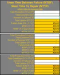
MTBF and MTTR
Project Pitfalls
Error Proofing
Z Scores
OEE
Takt Time
Line Balancing
Yield Metrics
Sampling Methods
Data Classification
Practice Exam
... and more