Normality Assumption

The normality assumption is an important topic in statistics since the vast majority of statistical tools were built theoretically upon this assumption.

There is always an element of error associated with statistical tools and the same applies to the normality assumption. It is virtually impossible to collect data from an exact normal distribution. However, many naturally occurring phenomena follow a very close approximate normal distribution. 

For example:

1-sample and 2-sample t-tests and Z-tests, along with the corresponding confidence intervals, assume that the data were sampled from populations having normal distributions. Most linear modeling procedures, such as Regression and ANOVA, also assume that the residuals (errors) from the model are normally distributed. In addition, the most widely used control charts and process capability statistics are based upon theoretical assumptions about the normality of the process data.

Since the assumption of normality is critical prior to using many statistical tools, it is often suggested that tests be run to check on the validity of this assumption. Keep in mind the following points: 

1.     Relative importance of the normality assumption

Most statistical tools that assume normality have additional assumptions. In the majority of cases the other assumptions are more important to the validity of the tool than the normality assumption. For example, most statistical tools are very robust to departures from normality, but it is critical that the data are collected independently.

2.     Type of non-normality

A normal distribution is symmetric, with a certain percentage of the data within 1 standard deviation, within 2 standard deviations, within 3 standard deviations, and so on. Departures from normality can mean that the data are not symmetric; however, this is not always the case. The data may be symmetric but the percentages of data within certain bounds do not match those for a normal distribution. Both of these will fail a test for normality but the second is much less serious than the first. 

3.     Data transformations

In many cases where the data do not fit a normal distribution, transformations exist that will make the data “more normal” and meet the assumptions of inferential statistics. The log transformation (or the Box-Cox power transformation) is very effective for skewed data. The arcsin transformation can be used for binomial proportions. The log transformation can be used to reduce the skewness of highly skewed distributions.

The Impact of Non-Normality

Non-normality affects the probability of making a wrong decision whether it is rejecting the null hypothesis when it is true (Type I error) or accepting the null hypothesis when it is false (Type II error).

The p-value (probability of making a Type I error) associated with most statistical tools is underestimated when the normality assumption is violated. In other words, the true p-value is somewhat larger than the reported p-value.

Assess the Data if Non-Normal

The following may be correctable methods or reasons for non-normal data:

1. Ensure you have gathered at enough data, especially with lower resolution.
2. Increase resolution (or granularity) of the measurements
3. A good representative sample has not been obtained and only a "short term" or subset is being analyzed that does not represent the entire process
4. Determine if outliers have assignable cause (special cause) and be removed. 
5. Ensure the data is not bi-modal or multi-modal. Varying inputs affecting the measurements during the data collection process should be minimized or eliminated.
6. If the data has tendency to approach zero, or some limit, then it will likely be skewed in that approached direction and thus will not be normal and a transformation may be needed. 

Normality Hypothesis Testing

Influencing Factors

The following factors impact the normality of the data:

Granularity - the levels of discrimination within the data measurements

Kurtosis

• Flatness (negative kurtosis)
• Peakedness (positive kurtosis)

Skewness - left-skewed, right-skewed, bi-modal, or multi-modal

Methods

The first step before using any statistical test that rely on the assumption of normal data is to determine if the data is normal. There are tests most often used:

1) "Fat-Pencil" Test

2) Normal Probability Plot

3) Anderson-Darling

4) Shapiro-Wilk

5) Ryan-Joiner

6) Kolmogorov-Smirnov

"Fat Pencil" Test

This is a visual judgment method to quickly get a general understanding of whether the sample data meets the assumptions of normality for the population from which the sample was collected.

The Fat Pencil test is one where a hypothetical wide line is drawn along the red line and if all the data points are contained within the line, then the data is assumed to be follow a normal distribution. 

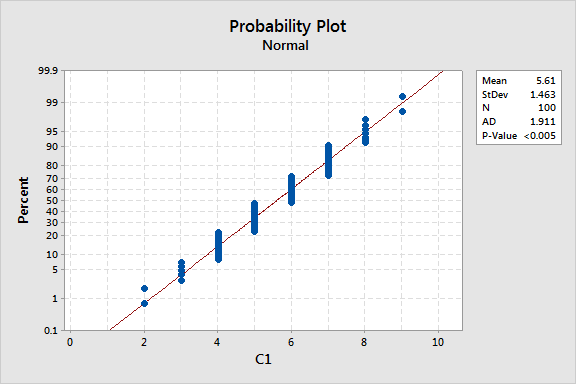
As you can see, depending on how "fat" the pencil is, one could conclude the data is normal. It is not extremely obvious that the data is non-normal. 

However, looking at the p-value that is <0.005, it is clearly not close to meeting the alpha-risk value of 0.05 (or even 0.01 if you are taking very low risk). 

So the data in this sample of 100 data points does not meet the assumption of normality for the population it represents. 

One of the factors that impacts normality is granularity or levels of measurement, sometimes referred to as discrimination. There are only 8 different responses and all 100 of them are whole numbers. Measuring to the tenths or hundreds is more ideal.

Normal Probability Plot

Another graphical method with more strength (meaning a better chance of making the correct decision) is the Normal Probability Plot. 

In this case the actual data is plotted and another line will show the perfectly normally distributed of data.

The z-scores along the x-axis are the expected z-scores if the data was perfectly normally distributed. 

If the data closely follows the theoretical line (which is the subjective part of your decision), and it does not go beyond 95% confidence interval lines (UCL and LCL), then the data can likely be assumed normal. 

Anderson-Darling

This statistic measures how well the sample data follow a particular distribution. The lower the value, the better the distribution fits the data. The test uses math to examine the skewness and kurtosis of the distribution.

The hypothesis for the Anderson-Darling test are:

   H_O: The data follow a specified distribution, such as a normal distribution. 

   H_A: The data do not follow a specified distribution, such as the normal distribution (indicating the data is non-normal)

When the p-value can mathematically being calculated, use the p-value to determine if the data come from the specified distribution.

The p-value is the probability that the sample data was selected from a normally distribution population. 

If the p-value is greater than the selected alpha-risk, the null hypothesis is inferred and the data do follow the specified distribution.

If the p-value is less than the selected alpha-risk, the null hypothesis is rejected and conclude that the data do not follow the specified distribution.

This method is considered the second strongest method of assessing normality behind the Shapiro-Wilk method. 

This method is generally slightly stronger than the Kilmogorov-Smirnov method since its critical values depend on the type of distribution of the data being tested and it gives more weight to the values in the lower and upper tails. 

For example: 

If the alpha-risk chosen is 0.05, and the p-value calculated using this method is 0.074, then the population can be assumed to follow a normal distribution. 

If the alpha-risk chosen is 0.05, and the p-value calculated using this method is 0.021, then the population can not be assumed to follow a normal distribution. Then, you should follow any possible correctable measures (read below) or consider a data transformation. 

The picture shown above, under the "Fat Pencil" test shows the p-value is <0.05 (a very commonly selected alpha-risk level), and there the null hypothesis is rejected and instead, the alternative is inferred which is the data do not follow the normal distribution. 

Using the Graphical Summary tool in Minitab, the histogram appears to follow nearly a perfectly normal distribution. However, statistically, the data does not meet the criteria and is non-normal. 

The point is to be careful - use both visual and statistical tools to assess the data. 

The p-value is much lower than the selected alpha-risk of 0.05. 

Ryan-Joiner

This test calculates a correlation coefficient using the following formula

IMAGE OF FORMULA

The closer the correlation coefficient is near to one, the closer the data is to the normal probability plot. If the correlation coefficient is lower than the appropriate critical value, reject the null hypothesis and the data can not be assumed to be normal.

Shapiro-Wilk

This testing method is considered the strongest or most robust normality testing method meaning that it correctly rejects the null hypothesis (meaning the HA is inferred and that the data does not have a normal distribution) more often than the other testing methods discussed here, especially with smaller sample sizes.

In this method, a statistic, W, is calculated. If this calculated test statistic is < than the critical value then the null hypothesis is rejected and alternative is inferred. 

The hypotheses for the Shapiro-Wilk test are:

   H_O: The data follow a specified distribution, such as a normal distribution.

   H_A: The data do not follow a specified distribution such as the normal distribution (indicating the data is non-normal)

Kolmogorov-Smirnov

In this method, the test examines the distance between the CDF of each data point in the sample to the true CDF of an exact normal distribution for that same data point. 

One more note about this test is that it is independent of the type of distribution being tested. The critical values are the same for any distribution type that is tested.

The hypotheses for the Kolmogorov-Smirnov test are:

   H_O: Distribution of actual data matches (equals) the distribution being tested which for this case means a normal distribution. 

When testing for normality, then the null hypothesis states the actual data match a normal distribution. 

   H_A: The data do not follow a specified distribution such as the normal distribution (indicating the data is non-normal).

Out of all the distances found with each data point and the true CDF for that data point, it is the largest distance that is compared to the critical value and a given sample size, "n", and selected alpha-risk level. 

When the distance is less than (<) the Kolmogorov-Smirnov critical value, the Ho is not rejected and, in this case, the data meets the assumption of normality. 

Parametric & Non-Parametric Tests

There are many non-parametric alternatives to standard statistical tests. However, these also assume that the underlying distributions are symmetric. Most standard statistical tools that assume normality will also work if the data is symmetric.

Also, consider that the power of the non-parametric tests only approaches the power of the standard parametric tests when the sample size is very large.

So, given the choice between the two, if the data are fairly symmetric, the standard parametric tests are better choices than the non-parametric alternatives.

Impact of Sample Size

For large samples (n >= 25), the effects of non-normality on the probabilities of making errors are minimized, due to the Central Limit Theorem. Sample size also affects the procedures used to test for normality, which can be very erratic for small samples.

Recall, that normality is assumed for the population, not the sample. When data is sampled from a population, it is often collected in small amounts of measurements relative to the entire population. This is another reason why the sampling plan is critical that is understood and done properly.

Six-Sigma-Material.com

Applicability within DMAIC cycle

ShareFacebookXWhatsApp

Measure Phase

In this phase, as for control charts, the effects of non-normality show up in the probabilities associated with falsely failing the tests for special causes. These effects are minimal for Xbar charts, even for very small (n < 5) subgroup sizes, provided the data are not extremely skewed. Even in cases of extremely skewed data, the effects are minimal if the subgroup size is 5 or more. 

Process capability indices themselves do not assume normality – they are simply ratios of distances. However, if one makes inferences about the defect rate based upon these indices, these inferences can be in error if the data are extremely skewed. One fortunate aspect of process capability studies is that it is standard practice to base them upon at least 100 observations, therefore lessening the impact of the normality assumption.

Analyze Phase

In this phase, the Six Sigma Project Manager must isolate variables which exert leverage on the CTQ. These leverage variables are uncovered through the use of various statistical tools designed to detect differences and patterns in means and variances.

Most of these tools assume normality. For many, there are non-parametric alternatives. As mentioned earlier, one should use good sense and judgement when deciding which test is more appropriate. It is a good idea to test for normality. If the test fails, check the symmetry of the data. With a large (n >= 25) sample, the parametric tools are better choices than the non-parametric alternatives, unless the data are excessively skewed.

Consider data transformations, especially when the data are skewed. Keep in mind that the p-values you see may be underestimated if the data are not from a normal distribution. The effect on the p-values is minimized for large samples.

If a standard parametric test is used and the reported p-value is marginally significant, then the actual p-value may be marginally insignificant. When using any statistical tool, one should always consider the practical significance of the result as well as the statistical significance of the result before passing final judgment.

Improve Phase

In the Improve Phase, the Six Sigma Project Manager will often use Design of Experiments (DOE) to make dramatic improvements in the performance of the CTQ. A designed experiment is a procedure for simultaneously altering all of the leverage variables discovered in the Analyze Phase and observing what effects these changes have on the CTQ.

The Six Sigma Project Manager must determine exactly which leverage variables are critical to improving the performance of the CTQ and establish settings for those critical variables.

In order to determine whether an effect from a leverage variable, or an interaction between 2 or more leverage variables, is statistically significant, the Six Sigma Project Manager will often utilize an ANOVA table, or a Pareto chart.

An ANOVA table displays p-values for assessing the statistical significance of model components. The Pareto chart of effects has a cutoff line to show which effects are statistically significant. 

All of these methods assume that the residuals after fitting the model are from a normal distribution. Keep in mind that these methods are pretty robust to non-normal data, but it would still be wise to check a histogram of the residuals to be sure there are no extreme departures from normality, or more importantly, are not excessively skewed.

If the data are heavily skewed, use a transformation. Also, bear in mind that the p-values in the ANOVA table may be slightly underestimated, and that the cutoff line in the Pareto chart is slightly higher than it should be. In other words, some effects that are observed to be marginally statistically significant could actually be marginally insignificant.

In any case where an effect is marginally significant, or marginally insignificant, from a statistical point of view, one should always ask whether it is of practical significance before passing final judgment.

Control Phase

In this phase the Six Sigma Project Manager generates a Control Plan for each of the critical leverage variables from the Improve Phase. These are the variables which truly drive the relationship Y = f(x₁,x₂,…,x_n). In order to maintain the gains in performance for the CTQ, or Y, the X (inputs) variables must be controlled. 

Control charts for continuous data assume the data are from a normal distribution, although control charts have been shown to be very robust to the assumption of normality, in particular the Xbar chart. A simulation study shows that even for subgroups of size 3, the Xbar chart is robust to non-normality except for excessively skewed data. For subgroups of size 5, the Xbar chart is robust even if the underlying data are excessively skewed.

If the I chart (subgroup size = 1) is used, the effects of non-normality will be seen in an elevated rate of false alarms from the tests for special causes. These tests are designed to have low probabilities of false alarms, based upon a normal distribution. As with the tools mentioned earlier, the data may be transformed, which is effective for skewed data. 

Checking for Normality in Minitab

There are a number of methods to assess normality in Minitab and most other statistical software and often, one tool itself, does not present the entire picture. Use a few tools combined to review the numbers and make conclusions.

A visual representation of the data such as through a histogram and probability plot is easy to generate and valuable to use in conjunction with the statistics. 

The screenshots below may vary depending on the version of Minitab but generally the path will remain similar. 

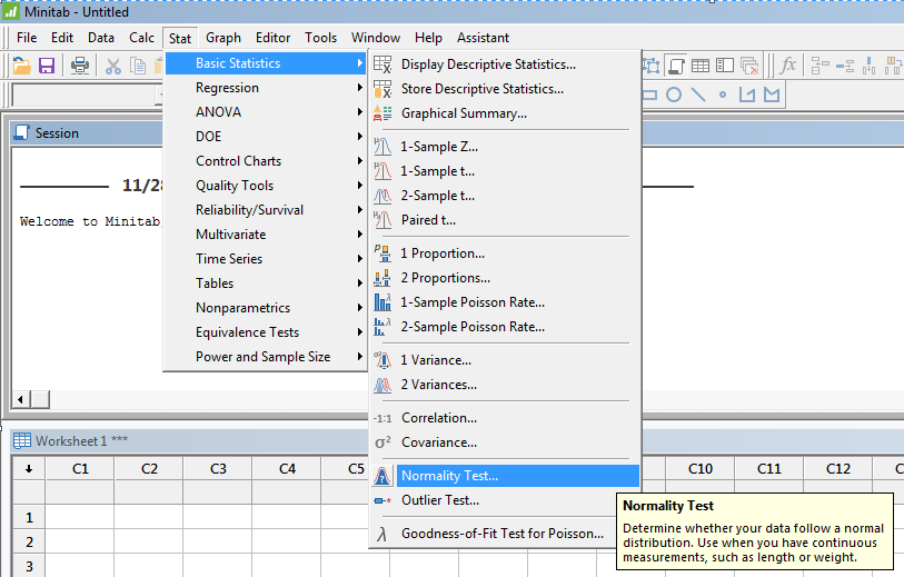
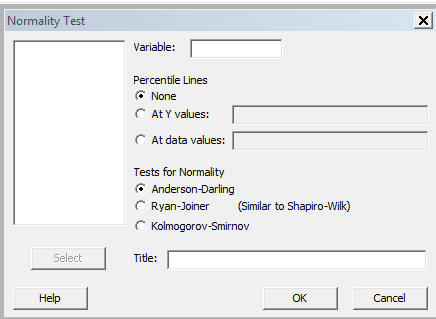
You can see that options are available to select from and this will likely be the case with most statistical software programs. 

This will generate a normality plot as shown above under the "Fat Pencil" test section. 

Summary

When using a statistical tool that assumes normality, test this assumption.

Use a normal probability plot, a statistical test, and a histogram. For large sample sizes, the data would have to be extremely skewed before there is cause for concern. For skewed data, try a data transformation technique.

With small samples, the risk of making the incorrect conclusion is increased with any tool, including the probability plot, the test for normality and the histogram.

Also, non-parametric alternatives have little discriminatory power with small samples. If using a statistical tool that assumes normality, and the test fails, remember that the p-value you see will be smaller than it actually should be.

This is only cause for concern when the p-value is marginally significant. For risk aversion, run the non-parametric alternative (if there is one) and see if the results agree. As with any statistical output, consider the practical significance and ensure the output seems realistic.

Return to the DEFINE phase

Return to the MEASURE phase

Templates and Calculators

Subscribe to access this entire site

Return to the Six-Sigma-Material.com home page