ShareFacebookXWhatsApp

Description:

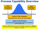
Proper data classification is the first step to ensure the correct statistical tools are used to analyze baseline and final performance.

Objective:

Six Sigma projects can start out with the wrong baseline sigma score or the improper control chart selection as a result of improper data classification. The goal is not only selecting the correct data type but to collect data that provides the most information at the least expense. There are four levels of data measurements: Nominal, Ordinal, Interval, and Ratio.

Six-Sigma-Material.com

Continuous (Variable) Data

Theoretically has an infinite number of measurements depending on the resolution of the measurement system. There are no limits to the gaps between the measurements. It is data that can be expressed on an infinitely divisible scale.

Even if the measurements range from 0-1 there may be an infinite number of measurements within (0.000000000000... to 0.999999999999...)

The continuous random variables can be any of the infinite number of values ​​over a given interval. These variables generally represent things that are measured, NOT counted.

Examples are:

• Temperature
• Height
• Money
• Weight
• Pressure
• Force
• Lumens
• Hardness
• Length
• Decibels
• Ohms
• Watts
• Amperage
• Voltage
• Torque
• Tension
• Distance
• Volume
• Area
• Tensile Strength
  

Discrete (Attribute) Data:

Data types that have a finite number of measurements and are based on counts. Data that can be sorted into distinct, countable, and in completely separate categories. The count value can not be divided further on an infinite scale with meaning.

Example: How many people can comfortably fit into an airplane? It does not make sense to say 129.7632213 people. It is either 129 or 130, in this case you would round down to 129. Attribute and discrete do not mean exactly the same when describing data, discrete has more than two outcomes.

• rating 1-10 (whole numbers with 1 being LOWEST - 10 being HIGHEST)
• ratings provided on an FMEA for Severity, Occurrence, and Detection
• color designation RED, BLUE, etc. (considered discrete categorical data)
• gender (considered discrete categorical data)
• race (considered discrete categorical data)
• # of defects on an order form or in a batch of parts
• political party affiliation (considered discrete categorical data)
• number of student or workers
• number of machines
• types of defects on an order form
• number of late deliveries
  

Bar graphs, pie charts, and Stem-and-Leaf plots are good choices for discrete data.

More about Attribute Data:

Used to represent the presence or lack of a certain characteristic. Discrete often refers to a "count" but may able related to an "attribute" characteristic.

A binomial measurement is the type of attribute measurement that has two characteristics. This is the lowest level of data type due to low level of information provided.

• go / no-go
• pass / fail
• on / off
• correct / incorrect
• full / empty
• hot / cold
• small / big
• paper / plastic
  

COMPARING DATA CLASSIFICATION TYPES

• Continuous data is more precise than discrete data.
• Continuous data provides more informative than discrete data.
• Continuous data can remove estimation and rounding of measurements.
• Continuous data often more time consuming to obtain.
  

NOTE: Convert to continuous data when possible as shown in the table below are a few examples to obtain a higher level of information and detail:

Six-Sigma-Material.com

Example One:

Instead of recording whether students PASS or FAILED the SAT, it would be better to have each student's actual score on the SAT.

Example Two:

Instead of a A Six Sigma Black Belt is looking to collect data on the timeliness of shipments.

• You could record each shipment as being late or on time (which is a binomial discrete data). This is a LOW level of measurement. It’s easier and quicker but provides minimal information.
• You may group each shipment as arriving 0-1 days early, 2-3 days early, 0-1 days late, 2-3 days late and so forth. This provides a little more data but still not ideal. Or groups such as Very Early, Early, On-Time, Late, or Very Late.

What would be ideal?

Each shipment should have a due date and possibly a specific time. That due date is the target. And each shipment has an actual arrival time.

From here, the performance of each shipment compared to its target delivery time can be calculated in days or possibly even hours.

Going left to right in the picture below, notice the data is more informative.

Also notice the performance seems to be worsening over time and is probably not normal. A lot of powerful information come with continuous data.

Example Three:

Instead of recording just the dollars or pieces scrapped, it is more valuable to know the scrap per unit or scrap per sales.

If Plant A had molding scrap cost of $63,000 / month and Plant B scraps $48,000 / month, which performed better? With a denominator such as sales dollars a better conclusion can be made.

If Plant A had $1,000,000 in sales in the same month, and Plant B had $50,000 in sales in the month, it is obvious that Plant B scrapped a much higher percentage of its product.

Or consider Scrap Pounds per Total Pounds Produced. And better yet, try to get both. One plant (or machine) may have a higher Scrap Rate in pounds but there scrap may be less expensive than the other plant (or machine). 

The more data the better so you can mine it several different ways. However, this take resources and time. 

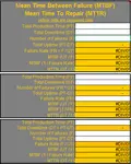
Take a look at the figure below. If you only collected the Scrap $, or the Scrap LBS, you would not have a complete picture of what is really happening among all 10 machines. 

All three columns are continuous values but adding a denominator (or ratio) provides you more information. See the takeaways at the bottom of each column. 

Machine 6 doesn't stand out as a problem when looking at only Scrap $ or Scrap LBS but it is clearly the most important to evaluate since it produces that most expensive scrap. 

Four Levels of Data Measurement

1. Nominal Data

The lowest level of data classification. A numerical label that represents a qualitative description. These numbers are labels or assignments of numbers that represent a category or classification.

This is also referred to a categorical data usually of more than two categories and is a form of discrete data and should apply nonparametric test to analyze. The number assignment does not reflect that one category is better or worse than another.

• Political Party Affiliation
  1 = Independent
  2 = Democratic
  3 = Republican


• Gender
  1 = Male
  2 = Female
  
  
• Geographical Location
  1 = Midwest
  2 = South
  3 = Northeast
  4 = East coast
  
• Marital Status
  1 = Single
  2 = Married
  3 = Divorced
  
  

The mode is the measure of central tendency.

Other types of variables that often result in nominal data are religion preference, zip code numbers, birth dates, telephone numbers, blood type, eye color, hair color, federal tax ID number, ethnicity, and social security numbers. There are limited statistical techniques to analyze this type of data, but chi-square statistic is most common.

The average of the data or variance of the data is meaningless and values ​​and quantitative descriptions are not appropriate. There is also no priority or rank based on these numbers.

For example, a birthdate of January 5th, 1935 is not better or worse than September 8th, 2012. Or blue eyes are not better or worse than brown eyes. 

2. Ordinal Data

The next level higher of data classification than nominal data. Numerical data where number is assigned to represent a qualitative description similar to nominal data. These are measures by only the rank order.

However, these numbers can be arranged to represent worst to best or vice-versa. Ordinal data is a form of discrete data and should apply non-parametric test for analysis.

• Ratings provided on an FMEA for Severity, Occurrence, and Detection
  
  DETECTION
  1 = detectable every time
  5 = detectable about 50% of the time
  10 = not detectable at all
  
  (All whole numbers from 1 - 10 represent levels of detection capability that are provided by team, customer, standards, or law)
  
  
• Classifying households as low income, middle-income, and high income
• Master Black, Black Belt, Green Belt, Yellow Belt, etc.
• Lower Class, Middle Class, Upper Class

Nominal and ordinal data are from imprecise measurements and are referred to as non metric data, sometime referred to as qualitative data.

The median or mode are measures of central tendency.

Ordinal data is sorted into categories and the categories can be put in a logical order but the intervals between categories is not defined.

Ordinal data is also round when ranking sports teams, ranking the best cities to live, most popular beaches, and survey questionnaires.

3. Interval Data

The next higher level of data classification. Numerical data where the data can be arranged in an order and the differences between the values ​​are meaningful but not necessarily a zero point. These are measures using equal intervals. 

Interval data can be both continuous and discrete. Zero degrees Fahrenheit does not mean it is the lowest point on the scale, it is just another point on the scale.

The lowest appropriate level for the mean is interval data. The mean, median, or mode are measures of central tendency.

Parametric AND nonparametric statistical techniques can be used to analyze interval data.

Examples are temperature readings in C or F (not Kelvin), percentage change in performance of machine, time of day, calendar days, and dollar change in price of oil / gallon, pH reading, age (if measured in years), SAT and ACT scores, and credit score

4. Ratio Data

Similar to interval data EXCEPT has a defined absolute zero point and is the highest level of data measurement. Ratio data can be both continuous and discrete.

Ratio level data has the highest level of usage and can be analyzed in more ways than the other three types of data.

The mean, median or mode are measures of central tendency.

Interval data and ratio data are considered metric data, also called quantitative data.

Examples include time, income, volume, weight, voltage, height, pieces / hour, force, defects per million opportunities, resistance, watts, per capita income, items sold, years of education, Kelvin, and lumens.

Please note that some measures (i.e. height) can be in more than one measurement scale. Height could be measured with Short, Medium, Tall but there is more information if measured to an exact centimeter or inch. 

Data Distributions

DISCRETE DISTRIBUTIONS:

1. Binomial Distribution
2. Poisson Distribution
3. Hypergeometric Distribution
   

CONTINUOUS DISTRIBUTIONS:

1. Uniform Distribution
2. Normal Distribution
3. Exponential Distribution
4. t Distribution
5. Chi-square Distribution
6. F Distribution
   

Return to the MEASURE phase

Link to newest Six Sigma Material

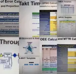
Templates, Tables, and Calculators

Return to Six-Sigma-Material Home Page