Power and Sample Size

Description

Show the relationship between Power and Sample Size. The Power of the comparison test refers to the likelihood the decision is made that there is a significant difference when it actually exist. Power represents the probability of rejecting a false null hypothesis.

Objective

The Power of a test determines if there's enough sensitivity to detect actual (true) differences. More power and sample size are necessary to detect smaller differences. Power quantifies the smallest difference the comparison test is capable of detecting.

Power = 1 - Beta Risk (Type II Error) = 1 - β

Confidence Level = 1 - Alpha Risk (Type I Error) = 1 - ∝

For example, if you want to have Power of 90% (or 0.90) you are saying you want to have at least a 90% chance of correctly rejecting the H_O (null hypothesis)

Inputs for determining Power

• Sample Size - you need this to calculate Power or on the reverse, you need the Power to determine the Sample Size. The best way to increase the Power is to increase the sample size. However this can be costly and time prohibitive.
• Alpha-risk - or critical p-value or Type I error you're willing to accept. A higher acceptable rate of false positives (or higher alpha-risk) increases the power. 
• Effects Size - measure of association (see test sensitivity below)
• Standard Error (SE)
• Sampling Design - or design effect

NOTE: The Confidence Level is different than the Confidence Interval. The Confidence Interval includes the Margin of Error which is the +/- figure usually found on scientific surveys and polls. 

---

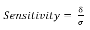
Test Sensitivity 

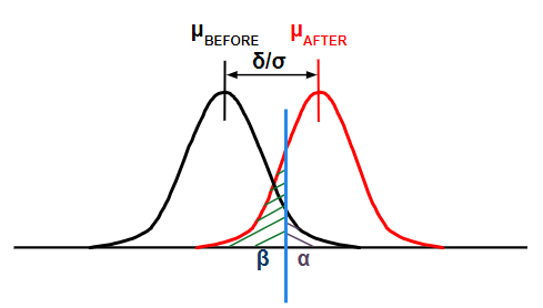
This is the relative size of the difference being tested denoted in standard deviations. The Power is calculated to determine if there is enough sensitivity in the statistical test to detect differences or effects when they exist.

As one would expect, more power (or lower beta-risk) is needed to detect smaller and smaller differences.

δ = size of difference

σ = standard deviations

the light blue line is the critical value. 

---

Type I Error

Type I Error = Alpha Risk = Significance Level = Producers Risk = False Positive.

This is a decision made that there is a difference when the truth is there is not. In other words, parts have been determined defective (possibly scrapped) and they were not defective. The Producer suffered by losing parts and needed to make up the lost inventory. 

Type II Error

Type II Error = Beta Risk = Consumers Risk = False Negative

This is when the decision is made that there is not a difference when the truth is there is a difference. In other words, parts have been determined not defective and sent to the customer (or downstream operation) and they were defective. The Consumer suffered by receiving defects.

---

Click here to learn more about alpha and beta risks

Recommended Video 

---

Margin of Error (ME) vs. Standard Error of the Mean (SE)

ME is often expressed as the following formula:

ME = critical value * Standard Error (SE)

The ME is also sometimes called the maximum error of estimate or error tolerance. The ME is the "radius" or half the width of the confidence interval for a distribution. 

The larger the ME, the less confidence that the results represent those of the entire population. The larger the sample size, the smaller ME. 

Ways to REDUCE the ME:

• Increase the sample size, n
• Decrease the Confidence Level (same as saying increase the alpha-risk,  ∝)
• Decrease the standard deviation 

For calculating the population standard deviation in the first formula you must know the population parameters.

For example, if there were thousands of customers surveyed for a particular contractor and we sifted through a sampling of 125 of them an found the average rating was 4.26 with a sample standard deviation of 0.21, calculate the Margin of Error for a 90% confidence level (or 0.10 alpha-risk = 10%)? 

The critical value is 1.645 for 90% CL

The standard deviation of the sample = 0.21. 

SE = the sample standard deviation / sqrt n = 0.21 / sqrt 125 = 0.21 / 11.18 = 0.01878 = SE

Therefore the ME = 1.645 * 0.01878 = 0.0309 = ME

Thus the center of the confidence interval, x bar, is the point estimate. Take the point estimate and subtract the ME for the lower bound of the CI and add the ME to the point estimate to the upper bound of the CI. 

The x bar value is 4.26%, then the CI = {4.26 - 0.0309, 4.26 + 0.0309} = {4.229, 4.291} 

In practical terms this means that you can be 90% certain that the population would choose a rating between 4.229 to 4.291 for that contractor.

If all things remain the same, the next result from the survey is 90% to have a result between 4.229 and 4.291. Obviously, most surveys don't ask for that level of resolution so there needs to be some reality check to the statistical answer. 

If you wanted a CL of 95% or 99%, the then margin for error increases since the critical value increase (in other words you want more confidence than 90% therefore you need to accept wider interval if you're going to keep the number of samples the same at 125). 

CLICK HERE to see a much more detail on Margin of Error with examples. 

---

Calculating Sample Size

The amount of samples to record in order to get the required output you want is dependent on a few factors:

1. The desired detection difference you want. Do you want to see any difference or do want to detect a certain amount of difference and in which direction?
2. The Confidence Level (or 1 - alpha-risk, ∝). Typically 95% is used (or 5% alpha-risk)
3. The level of Power (or 1 - beta-risk, β)
4. The level of variability (variance) or standard deviation 

There are many tutorials and calculators on the web. A few links/videos are shown below:

https://www.surveymonkey.com/mp/sample-size-calculator/

https://www.surveysystem.com/sscalc.htm

https://www.calculator.net/sample-size-calculator.html

---

Sample Size Calculation - Variable Data

Determine the sample size needed to detect a mean shift of 0.049 on a process with standard deviation of 0.03924.

Assume the data is from a normal distribution.

Use alpha-risk of 5% and beta-risk of 10%. Therefore the CL is 95% (1-0.05) and the Power is 90% (1-0.10)

The mean of one set of 40 samples from a normally distributed set of data was 0.430 and the mean from another set of 40 samples from a normally distributed set of data was 0.381.

Summary:

From the top picture, notice that 15 samples were needed to detect difference of 0.049 at a Power of 90%. From the bottom picture, notice the true Power is >99% since the sample size was actually 40.

Keep in mind this example focuses on statistically detecting a shift in the mean. This does not indicate anything about the variation between the two sets of data. If this were a before and after analysis, it is possible the variation increased after while still shifting the mean favorably.

The emphasis of Six Sigma is on variation reduction and the F-test is used in this case (normal data) to determine if there is a statistical change in the variation.

More about SAMPLE SIZES

Learn more about calculating Samples Sizes for Variable, Poisson, and Binomial data by clicking here.

---

Return to BASIC STATISTICS

Return to the ANALYZE Phase

Return to Surveys

Accelerate your Six Sigma Project

Return to the Six-Sigma-Material Home page