Multi-vari Studies

Families of Variation

Multi-vari analysis is applied in the beginning of the ANALYZE phase to reduce the focus from all inputs (x's) creating the variation to a much smaller group of variables. Use Multi-vari studies among the FOV's to find specific areas to hone in.

Take this example below. The MSA has passed at this point and the Study Variation has been quantified. The remaining variation of the total is related to the PROCESS.

This is NOT the same as multivariate analysis.

Six-Sigma-Material.com

Within the process, the team found came up with 5 sources of variation to examine. The GB/BB then ran Multi-Vari charts with ANOVA tests on four of the sources and used F-test and 2 sample t-test on another source.

From here the data found a significant source of variation from Plant to Plant. Within that, it was found that Plant C was highest contributor to variation.

The GB/BB continued to mine the data further to examine the same original FOV's with only Plant C. At this point, the GB/BB may have found that certain machines, operators, a particular part, or a shift was the primary contributor.

Recall, the focus of Six Sigma is on VARIATION reduction, not only shifting the mean. This could even result is slightly reducing the performance of the mean if it results in drastically reduced variation.

If there was Machine A that ran an average of 23,492 pcs/hr with a standard deviation of 4891 pcs/hr and Machine B that ran an average of 23,400 pcs/hr with a standard deviation of 10 pcs/hr then the latter is probably preferred.

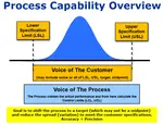
Although both are important the team's goal is to stabilize and make the process more repeatable, controlled, and predictable before trying to shift the mean to a more desirable target. In other words, make the process more PRECISE before making the process more ACCURATE but ultimately both are desired.

The purpose of FOV

Almost every set long term data contains rational subgroups. It is very important that a GB/BB understands how to dissect the data to understand the variation created by the families of variation.

Remember, by this stage the Measurement System variation has been quantified and the remaining variation is the Process Variation.

Each subgroup being analyzed contributes to the total Process Variation. The key is to analyze the FOV to identify the vital few inputs (KPIV's) that are creating most of the process variation.

Quantifying and visually showing the team members the magnitude of the variation created by each of the subgroups is extremely relevant to the team so they can focus on right areas to reduce variation and improve the mean.

Frequently it isn't as simple as that, and variables can have interaction and confounding effects on one another where a DOE becomes important.

Using simple Multi-vari Charts

These charts are a graphical method of presenting ANOVA (analysis of variance) data in comprehensive visual manner. These charts are often used to gain a qualitative understanding of the input (x's) contributions on the process and interactions of the inputs prior to more time-consuming numerical analysis.

Team members tend to find these charts easier to grasp than statistical results and often have a deeper level of interest in the data when it is presented in this format.

The chart displays the means at each factor level for every factor but also show the spread of the data. They are quick and inexpensive to generate with a potential high reward of discovering something lurking in the data.

Multi-vari charts are a graphical representation of potential Key Process Input Variables (KPIV's) and their relationship to the Effects (Y's). They are used to drill down into the "vital few" inputs that are creating most of the variation and then the team can focus on the highest impact improvements.

Multi-vari studies classify variation sources* as:

Positional – variation within a single unit (or piece)
Cyclical – variation between (among) unit-to-unit repetition over short time period
Temporal – variation over longer periods of time (drifts, trends)

*Material variation is sometimes cited as another key variation source, but Six Sigma certification questions are usually looking for Positional, Cyclical, and/or Temporal.

It is not so important to categorize into one of the above but more important to recognize and study the sources of variation in as many ways as possible.

As mentioned earlier, multi-vari charts are generally inexpensive ways to find quick insight about where, and where not, to focus improvement efforts. Other methods such as surveys and SPC can take more resources to find this same information. There is no reason a GB/BB should not take the time to run these charts.

The analysis is easy and quick once you get familiar with the software; the data collection, organization, is hard and time consuming. Putting the hard work up front to collect enough, meaningful data, will pay dividends as you proceed to the IMPROVE phase.

You will know where to prioritize improvements to get the most for your resources. You can't fix everything...tackle the vital few sources of variation.

The Process

1) Create the Families of Variation tree (which are rational sub-groups making up the Process Variation). Such as:

part-part, piece-piece
shift-shift,
machine-machine,
form-form,
lot-lot,
batch-batch,
facility-facility,
operator-operator,
tool-tool,
mold-mold,
month-month
heat-heat,
supplier-supplier,
house-house,
car-car
across length, or top to bottom of a piece (form of positional variation)
across width of a piece (form of positional variation)

Determine which rational subgroups will show relationships and interactions of the key inputs.

2) Use as many graphical techniques as possible, within reason, to illustrate sources of variation (such as Boxplots, Scatter Plots, SPC, etc.).

3) Create Multi-Vari charts for all of three. This will eliminate subjective reasons or validate them and help to show relative impact of the sources. This helps a GB/BB narrow their statistical tests to a smaller set of variables.

4) Analyze the graphs. What are they telling you?

You may need to collect more data where you suspect there is a lot of variation and narrow that collection to the suspect groups and try to confirm the results. Remember a good sampling plan ensures that a broad spectrum of data is collected that includes relevant sources of variation noise.

In other words, collect data on several lots, batches, shifts, machines, tools, etc. Depending on how easy and economical the data can be collected, strive to get as much as possible within each rational subgroup.

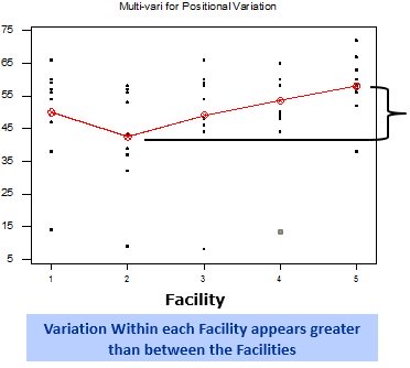
Positional

The chart below helps visualize the relative consistent from facility-to-facility but the variation is wide within each facility. The variation among facilities appears to be less of a concern (see the spread of the red line) than the variation within some of the facilities (see the spread of the data points within each facility).

ANOVA will quantify the variation between facilities and within facilities to confirm the graph. The graph is more powerful to show the team, the statistics are your friend as the proof.

An F-value of the Facilities that is below the F-critical value indicates the variation within the Facilities is greater than the variation between them. The opposite is true if the F-value is greater than the F-critical value.

A more discriminate investigation of positional variation may include examining mold-mold variation within a particular facility, or press-press variation within a particular facility.

About Multi-vari Charts

MULTI-VARI CHART show the following three categories of which can reflect process time related elements.

1) Cyclical (such as Batch to Batch, Lot to Lot, Piece to Piece)

2) Temporal (time comparisons)

3) Positional (such as across width or across the diameter)

Cyclical

These sources of variation are between (or among) unit-to-unit repetition over a short time period such as:

1st Shift - 2nd Shift - 3rd Shift
Lot to Lot (within a shift, or an hour)
Hour to Hour

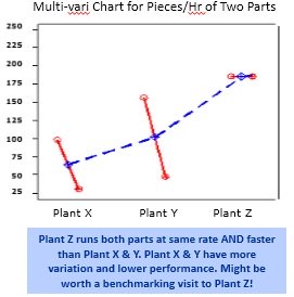
There are 3 factors (Plant X, Y, and Z) and 2 levels (Part 1 and Part 2). The y-axis is the pieces/hr that each part ran at (the output) at the respective plants. The blue dots are the mean values (in pieces/hr) of the two parts at each plant.

Temporal

These are sources of variation that occur over periods of time (time frames). With this type of analysis, the goal is to identify drifts or trends related to time events such as:

Hour-Hour
Day-Day
Week-Week
Winter-Spring-Summer-Fall
Month to Month....
Q1-Q2-Q3-Q4

The chart indicates a more consistent output at 1PM than the other two times (tighter spread) but efficiency Is declining from 10AM to 3PM with a few concerning low outliers at 3PM.

A F-test for variances will like not pass as the three times frames visually appear to have significantly different variation.

Perhaps the low outlier at 10AM and two lower three lower outliers at 3PM are false reading (or special cause). Removing them would show a fairly similar mean and variance for all three time frames.

Multi-vari Study - Download

Click here to a .pdf presentation with over 1,000 slides on multi-vari analysis and other Six Sigma and Lean Manufacturing principles...plus a 180+ practice certification questions.

Limitations

Multi-vari studies have limitations as do most tools. Understanding these and the pitfalls within each tool are important for a GB/BB.

The following are a list of potential pitfalls using multi-vari studies:

Confounding of input is present or multicollinearity. A DOE should be performed to further examine the interactions of the inputs.
Interactions may exist within the data but are not shown with studying one "x" at a time.
The data collected may be too narrow of a range and not represent all the proper input "x's" behaviors that influence "Y", the output.

Return to the ANALYZE phase

Search for Six Sigma related job openings

Templates, Tables, and Calculators

Return to the HOME page