ShareFacebookXWhatsAppReddit

Chi-square distribution

There are three primary types of Chi-square tests:

1. Independence
2. Goodness of fit
3. Homogeneity

The Chi square distribution is a measure of difference between actual (observed) counts and expected counts. There are several types of chi square tests, this module reviews a couple of the most common tests.

1. Chi square test for independence in a "Row x Column" contingency table.
2. Chi square test to determine if the standard deviation of a population is equal to a specified value.

Unlike the normal distribution, the chi-square distribution is not symmetric. Separate tables exist for the upper and lower tails of the distribution.

The most common Goodness of Fit tests are the chi square test which can be used for discrete distributions such as the binomial and Poisson distributions. The Kolmogorov-Smirnov and Anderson-Darling Goodness of Fit tests can only be used for continuous distributions.

This statistical test can be used to examine the hypothesis of independence between two attribute variables and determine if the attribute variables are related and fit a certain probability distribution.

The figure below shows an example of a non-symmetric chi square distribution with the p-value representing the area of the rejection region under the curve that is greater than the test statistic. This example would be a one-tail test.

Assumptions for using these chi-square tests

• Chi-square is the underlying distribution for these tests
• Attribute data (X data and Y data are attribute)
• Observations must be independent (if the data is paired or dependent, use the McNemar's Test which test for consistency in responses of two variables rather than their independence. This test can only be applied on 2*2 table)
  
• Works best with ≥ 5 expected observations in ≥ 75% of the cells (if If there are ≥ 5 expected observations in < 75% of the cells, use Fisher’s Exact Test) 

Ideally used when comparing more than two samples otherwise use the 2-Proportions Test (with two samples) or 1-Proportion Test (with one sample).

See Hypothesis Test Flow Chart as a reference. 

Chi-square formula for test of independence

The sum of the expected frequencies is always equal to the sum of the observed frequencies. The chi-squared statistic can be used to:

1. Test if a distribution is a good fit for population (Goodness-of-Fit)
2. Test association of two attribute variables (Test for Independence)
   

Chi-square Applications

• Test to see if a particular region of the country is an important factor in the number wins for a soccer team
• Determine if the number of injuries among a few facilities is different
• Determine if the types of TV channels watched are identical between males and females
• Determine if a coin or a set of dice is biased or fair.

Goodness of Fit (GOF) Hypothesis Test

The GOF test compares the frequency of occurrence from an observed sample to the expected frequency from the hypothesized distribution.

As in all hypothesis tests, craft a statement (without numbers) using simple terms for the team's understanding and then create the numerical or statistical version of the problem statement.

• State the practical problem
• State the statistical problem
• Develop null and alternative hypotheses
• Create table of observed and expected frequencies
• Calculate the test statistic or p-value
  

The Degrees of Freedom = (# of Rows - 1) * (# of Columns - 1)

Two methods can be applied to test the hypotheses. The decision to reject the null (and infer the alternative hypothesis) if:

1. Calculate the critical value the chi-squared test statistic and reject the null hypothesis if the calculated value is GREATER THAN the critical value
   
   OR
2. Reject the null hypothesis if the p-value is LESS THAN the alpha-risk. For a Confidence Level of 95% the alpha-risk = 5% or 0.05.

Chi-square in Excel

Using Excel to determine the p-value is done by:

P-value = CHISQ.TEST(Observed Range, Expected Range)

Excel asks for the "Actual" range which is the "Observed" range.

See the table below of the Observed values, Expected Values, and each chi-square value calculated using the formula above. The sums of all of them is the total chi-square statistic.

If the Level of Confidence is 95% (alpha risk = 0.05), then the p-value calculated above is > than 0.05.

The decision is to fail to reject the null hypothesis and to infer the null hypothesis. There is insufficient evidence that results are not due to random chance.

Test for Independence

Tests the hypothesis of independence between two attribute variables. The test does not require an assumption of normality.

dF = (# of Rows - 1) * (# of Columns - 1)

As in all hypothesis tests, craft a statement (without numbers) using simple terms for the team's understanding and then create the numerical or statistical version of the problem statement.

• State the practical problem - Is Y variable independent of the X variable
• State the statistical problem
• Develop null and alternative hypotheses.
• H_O: Y is INDEPENDENT of X (no difference)
• H_A: Y is DEPENDENT of X and at least on combination is different
• Create table of observed and expected frequencies
• Calculate the test statistic or p-value

Translate the statistical results into the practical result.

Observed and Expected Values of Attribute Data

Create the table of Observed values and create the table of Expected values.

Creating a table helps visualize the values and ensure each condition is calculated correctly and then the sum of those is equal to actual chi-square calculated value.

This also helps to understand how difference observed values can affect the results of the test. In the example above, a small change in one or a couple of the data points (a higher separation between the observed and expected value) can create a p-value less than 0.05. 

Calculate Expected values for each condition (fe).

f_e = (row total * column total) / grand total.

The chi-square calculated value is compared to the chi-square critical value depending on the Confidence Level desired (usually 95% which is alpha-risk of 5% or 0.05)

Example Test for Independence

Notice that the example begins with the table to help visually explain the problem and makes it easier to follow the problem solving process. 

Chi-square test for Variance

As mentioned at the top of this page, the chi square test can be used to test if the variance of a population (σ²) is equal to a specified or target variance (σ_t²).

NOTE:

For a 1-sample Chi-square Variance Population Test the assumption of normality must be met with the population or at least the sample. Having >30 samples typically waives the requirement for t-tests but does not waive the requirement for this test. 

If the data can not be assumed normal, Levene's Test and the Brown-Forsythe Test are two nonparametric alternatives. 

Hypothesis Test:

H_O: σ² = σ_t²  (in other words the variance of the population equals the target variance or specified variance. Or the new population variance is the same as the old population variance before changes were made, such as improvement by the Six Sigma team)

H_A: σ² < σ_t²   for a lower one-tailed test or

H_A: σ² > σ_t²   for an upper one-tailed test or

H_A: σ² ≠ σ_t²   for a two-tailed test

The chi-square test statistic formula (χ_t): 

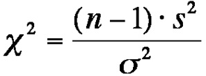
n = sample size and s = sample standard deviation

dF = n-1

s = sample standard deviation (s² = sample variance)

The null hypothesis (H_O) is rejected if:

• For lower one-tailed test: T < Chi-square critical value
• For upper one-tailed test: T > Chi-square critical value
• For two-tailed test: T > or < Chi-square critical value

EXAMPLE

25 measurements were gathered from a widget and have a variance of 0.03 mm. Test the null hypothesis that the true variance is 0.02 mm. Assume a 95% Confidence Level.

Solve:

H_O: σ² = 0.02 mm

H_A: σ² ≠ 0.02 mm therefore a two-tailed test

n = 25

Sample variance (s²) = 0.03 mm

dF = n-1 = 25-1 = 24

Significance Level: α = 1 - CL = 1 - 0.95 = 0.05

Chi-square test statistic (χ_t): = (n-1) (s/σ_t)² = (25-1) (0.03² / 0.02²)

= 24 (2.25) = 54.00

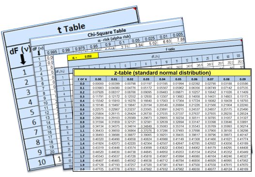
Use the table below carefully to find the rejection regions (two regions in this case). This is a two-tailed test with a significance level of 0.05; therefore each tail will contain half of the rejection region. 

Now look at the 0.975 column AND 0.025 column to find the respective starting points for the rejection regions on each side of the chi square distribution. 

So, the rejection region is any value < 12.401 and > 39.36. That total area is 0.05 of the chi square distribution. 

The calculated test statistic is greater than the critical value (54 > 39.36). The calculated test statistic falls WITHIN a rejection region. 

There the null hypothesis is rejected and the alternative is inferred which means the variance is different than the true variance.

Example quiz questions

These questions have been known to appear on statistics and Six Sigma quizzes. What test best fits the process/statement described below:

1) Does the data validate the normal probability distribution assumption?

2) Data were gathered in an experiment comparing the effects of three insecticides in controlling a certain species of parasitic beetle. Each observation represents the number of such insects found dead in a certain fixed area treated with an insecticide.

3) Do contingency table classification values matter? 

4) A multinomial probability distribution describes the distribution of counts across multiple levels of a variable. A special case is the binomial discrete probability distribution. For each level of a variable which is common to multiple populations, equality of distributions can be tested. 

Answers:

1) Comparing data to see how well it fits the normal distribution: Chi-square goodness-of-fit

2) Comparing average of >2 effects: ANOVA

3) Comparing factor association: Chi-square test for independence

4) Comparing distribution of frequency counts: Chi-square test for homogeneity

Chi-square Table

Statistical tables, including chi-square, z, t, and f tables, are available to download along with several more Templates and Calculators. Click here to review.

Chi-square "Goodness of Fit" on TI-83/84 Calculator

Chi-square "Independence" Test on TI-84 Calculator

Return to BASIC STATISTICS

Return to the ANALYZE phase

Search Six Sigma related job openings

Return to the Six-Sigma-Material home page