|

 content.")
Regression
Regression and correlation are similar in that they both involve testing a relationship of two continuous variables rather than testing of means or variances.
Both are used to find out the variables and to the degree the impact the response so that the team can control the key inputs. Controlling these key inputs is necessary to shift the mean and reduce variation of an overall Project "Y".
Regression analysis is a set of statistical processes for estimating the relationships between a dependent variable, often referred to as the "outcome variable" and one or more independent variables often referred to as the "predictors".
Recall that the Correlation coefficient (COC) indicates the amount of linear association that exists between two quantitative variables with a value between -1.0 to 1.0. An example value of -0.2636 indicates a weak negative correlation.
Regression provides an equation describing the nature of relationship such as
y = mx + b
where m is the slope of this equation. This is most commonly used formula but not always the best fit. In this case, m, represents the slope (rise/run or change in Y per change in X). And, b, represents the y-intercept or where the line crosses at x = 0.
Assumption:
Continuous data with interval or ratio measurement level.
Applications:
- Is there a (and quantify) relationship equation between driving speed and fuel consumption?
- Is there a relationship between money spent on commercials and product sales?
- Is there a relationship between training and job performance?
- Predicting the number of items and consumer will probably purchase.
- Analyze call center wait times to the number of complaints.
- Evaluate trends, make estimates, and forecasts (predictions).
Jargon:
Response Variable - dependent, uncontrolled, "Y", output variable, outcome variable.
Regressor Variable(s) - independent, controlled, "X" variables, input variables, which affect the Response. Often called "predictors" or "features"
Noise Variable - input variables that are not controlled
Regression Equation - describes nature of the relationship between independent variables and dependent variable
Residuals - difference between predicted response values and observed response values. These are assessed for normality to ensure the equation is applicable.
There are various types of Regression:
Simple Linear Regression
Single regressor (x) variable such as x1 and model linear with respect to coefficients. This is the most common form of regression analysis.
Multiple Linear Regression
Multiple regressor (x) variables such as x1, x2...xn and model linear with respect to coefficients.
Simple Non-Linear Regression
Single regressor (x) variable such as x and model non-linear with respect to coefficients.
Multiple Non-Linear Regression
Multiple regressor (x) variables such as x1, x2...xn and model nonlinear with respect to coefficients.
What is R-squared?
R2 refers to quantity of Y variation explained due to model. This represent a % of the variation in "Y" that can be explained by variation in the input variable (remember only testing this one input variable).
R2 = variance explained by the model / total variance
It is possible to have a p-value below 0.05 however the R2 value is also relatively low which indicates there are other inputs and sources of variation (x’s) that should be included in the model.
Typically, larger R2 values represent a regression model that better fits the data (or your observations). However, there are limitations to R2 to be mindful of:
A biased model can have a low or high R2 value. If the R2 value is low, you may still have a good regression model.
Vice versa, you may think the high R2 represents a strong regression model but in fact it isn't. And vice versa, you may think the high R2 represents a strong regression model but in fact it isn’t. It could be purely coincidental….so thinking is required to rationalize the outcome (as in all statistics).
R2 is unable to determine if predictions are biased which is a reason for examining the residuals which is explained later.
Remember that its valid for the range of data analyzed and any data outside (above or below) could change the true regression model and R2 value.
All of these formulas below are different ways to calculate R2 if you have the SS (Sum of Squares) values.
A) R2 = SSregression/ SStotal
B) R2 = (SStotal - SSerror) / SStotal
C) R2 = 1 - [SSerror / SStotal]
The SStotal = SSregression + SSerror
Regression - Example
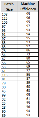
A Six Sigma Black Belt is interested in the relationship of the (input) Batch Size and its impact on the output of Machine Efficiency. The
- Predictor variable (x) is the Batch Size, and the
- Response variable (output) is the Machine Efficiency.
The following data was gathered with as much caution to keep other variables constant. The same part number was ran on the same machine with the same operator under similar operating conditions.
The data can be in any order and does not have to be normal (the residuals should be normal but the data itself does not have to be normal).
Notice the minimum input batch size trialed was 25 and the maximum is 115. Therefore the inference range for any regression formula would be from 25 to 115.
The data was modeled with a Linear, Cubic, and Quadratic fitted line. See the charts below.
The initial scatter diagram (without any fitted line) isn't obvious that the relationship may not be best explained with linear fitted line plot, so the Black Belt decides to model the data in various ways.
Notice the best fit is with the Quadratic fitted line plot that has an R2 value of nearly 97.9%.
Recall, the R2 value will be in a range from 0% - 100%. This represents the % of explained variation. This is the % variation of the y-values that are explained by the linear relationship with x.
Linear Fitted Line Plot

Quadratic Fitted Line Plot

Cubic Fitted Line Plot

There are a few important points and takeaways from the results.
- The Cubic Fitted Line Plot has highest R2 fit.
- The formula can be used to assess outcomes based on the inference space (or batch sizes) from the lowest batch size to the largest.
- Also, adding the Confidence Intervals and Predictor Intervals at 95% (see below) can help the team determine most likely best- and worst-case scenarios. Obviously, the machine efficiency can never exceed 100%.
- Once the Batch Size reaches ~80 the Machine Efficiency gains begin to slow down then plateau around a batch size of 100.
- The greatest improvement (greatest upward slope) is start with batch sizes from ~40 to ~80 then the efficiency gains slow down (but do continue to increase) to near 95% at 100.
- If the inventory is justified, produce in batches of about 100 to maximize the efficiency of the machine without creating excess inventory (remember that not all inventory is bad).
Producing in larger batches contradicts Lean principles and the objective to get to "one-piece flow" however it may be the most Economic Order Quantity (EOQ) for the business.
Every decision has pros/cons and can improve some metrics and hurt others. It's important for the team to weigh the pros/cons and get consensus.
Produce in larger batches if approved and necessary. Determine the EOQ and get consensus. Then focus on SMED and reducing the reasons to increase batch sizes in the first place. Continue to push for smaller batches but only AFTER improvements have been made and proven to justify a lower EOQ.
When those efforts are complete and the team has agreed that the reasons for increasing batches are all addressed with improvements in place, then batch sizes can be justified with buy in from management.
NOTE on the EOQ:
Remember, the EOQ for one operation may not be the best for the overall value stream. You must consider all the operations, movements, freight, etc. All too often, we see examples of an EOQ for one operation being set and it is not the optimal for several of the downstream operations. So, one is fixed, and the others get worse. Be careful to avoid this type of decision.
Click here to get an EOQ Calculator (and many others)

Statistical Analysis in Minitab
Using the 'Method of Least Squares' which determines a line minimizes the sum of squares of residuals.
Using the p-value refers to the hypothesis test of the slope of the best fit line. The p-value is the probability that the slope is significant.
If the p-value is < alpha risk (usually 0.05) then the regression is statistical significant and X is linearly related to Y.
- HO: Regression model is not significant
- HA: Regression model is significant and can be used with the data range.
Use the 95% prediction bands as shown in the example below. With 95% confidence the response "Y "with input "X" will fall within the 95% prediction band range.
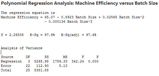
The best equation to use to predict the efficiency is of batch sizes between 25 and 115 is:
Y = 65.07 - 0.8923X + 0.02565X2 - 0.000136X3
The p-value is 0.000 which is < alpha risk of 0.05 so the equation can be used to model estimations within the inference range.
R2 = SSRegression / SSTotal = 5268.98 / 5381.88
R2 = 0.979 = 97.9%.
INFERENCE RANGE:
Think about the inference range and why it is critical. The inference range is from the minimum value of 25 to the maximum value of 115.
This means that you can apply this cubic formula to any batch size (x) to predict the machine efficiency.
If the batch size is 0, then Y would equal 65.07% machine efficiency. This is obviously not possible or realistic.
If the Batch Size was 1, this still represents an unrealistic output. So, it is important to use the Regression equation only within the Inference Range of 25 to 115 in this case.
Use the 95% prediction bands as shown in the example below. With 95% confidence the response "Y "with input "X" will fall within the 95% prediction band range.
Example:
The Finance Dept. has determined the EOQ to be a batch size of 65 since the cost of extra inventory is too great and there isn't ample storage space.
What is the Machine Efficiency at a Batch Size of 65?
Y = 65.07 - 0.8923(65) + 0.02565(652) - 0.000136(653)
Y = 65.07 - 57.9995 + 108.37125 - 37.349
Y = 78.09%
You can expect the Machine Efficiency to be about 78%.
Gut check: Looking at the red line and x-axis value of 65 goes up to about a y-axis value of 78% so this looks correct.
Remember, this formula is only valid for x values from 25 to 115. In other words, you can "infer" this prediction using any value from batch sizes from 25 to 115 only!
If you decide to input batch sizes <25 and >115 you are taking a chance of the prediction formula not being correct. Be careful...sometimes it works and sometimes it does not.
Assumptions for using Regression
Before performing a complete regression study there are assumptions about residuals must be satisfied. Residuals represent the error in the fit of regression line and is difference between the observed value of response variable and best fit value
The residuals must be:
- independent
- follow a normal distribution (or be able to assume normality), mean of 0.
- with equal variance
Statistical software programs often have the capability of handling these reviews to determine whether the regression results can be used.
In the above, "Fitted Linear chart, a residual is the difference in the blue dot from the red fitted line.
Regression and Correlation Download
 |
This module of slides provides additional insight into Correlation and Regression. This is critical component of statistical analysis and can quickly provide answers about the inputs and their effect on the outputs. These tools are frequently used in the DMAIC journey. Click here to purchase the Correlation and Regression module and view others that are available. |
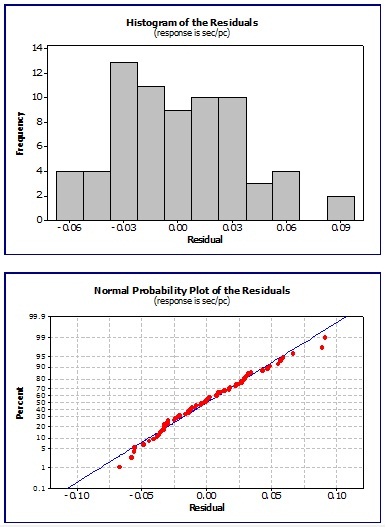
Example of Residual Testing
The charts below are typical results using a software program to analyze the residuals which are the error in the fit of the regression line.
This is the difference between the observed value of the response variable and fitted value.
Examining a set of data, the visual results of the residuals are shown below.
The behavior appears to be independent, normal, and exhibit random behavior which is acceptable to proceed with developing a regression equation.
The top two charts show the residuals do not exhibit any obvious trends or patters. They follow a random distribution with equal variance
The bottom two charts of the histogram and "fat pencil" normality test indicate roughly that the residuals resemble a normal distribution.
If all the assumptions PASS, then the regression model is valid.

However, there may be instances where the residuals indicate an underlying behavior that needs further evaluation.
If there is a:
Pattern or Trend: Likely another underlying input variable that needs to be separated or studied further for its impact.
Outlier: Examine each case of special cause and correct or explain.
Non-normal distribution: There may be bi-modal or other skewness with data that requires further understanding.
In any event, you and the team will learn more by having this discussion. It is important not to ignore the residual evaluation. It is better to understand the lurking variables and special causes now in order to make appropriate improvements and prevent surprises in the CONTROL phase.
Another Example using Minitab
A couple screenshots inputting the data into Minitab and selecting the Cubic fitted line. It is statistically significant at an alpha risk of 0.05 (5%) or confidence level of 95% since the P value = 0.000


The higher, the stronger the correlation. R2 in the example output below is 85%.
Added the Confidence and Predictor Intervals as well.

Recent Articles
-
Process Capability Indices
Oct 18, 21 09:32 AM
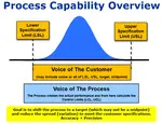 Determing the process capability indices, Pp, Ppk, Cp, Cpk, Cpm
 -
Six Sigma Calculator, Statistics Tables, and Six Sigma Templates
Sep 14, 21 09:19 AM
 Six Sigma Calculators, Statistics Tables, and Six Sigma Templates to make your job easier as a Six Sigma Project Manager
 -
Six Sigma Templates, Statistics Tables, and Six Sigma Calculators
Aug 16, 21 01:25 PM
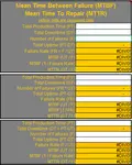
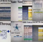
Six Sigma Templates, Tables, and Calculators. MTBF, MTTR, A3, EOQ, 5S, 5 WHY, DPMO, FMEA, SIPOC, RTY, DMAIC Contract, OEE, Value Stream Map, Pugh Matrix -
Six Sigma, Six Sigma Training, Courses, Calculators, Certification
Aug 15, 21 10:27 PM
 One site with the most common Six Sigma material, videos, examples, calculators, courses, and certification.

Site Membership
LEARN MORE
Six Sigma
Templates, Tables & Calculators
Six Sigma Slides
Green Belt Program (1,000+ Slides)
Basic Statistics
Cost of Quality
SPC
Control Charts
Process Mapping
Capability Studies
MSA
SIPOC
Cause & Effect Matrix
FMEA
Multivariate Analysis
Central Limit Theorem
Confidence Intervals
Hypothesis Testing
Normality
T Tests
1-Way ANOVA
Chi-Square
Correlation
Regression
Control Plan
Kaizen
MTBF and MTTR
Project Pitfalls
Error Proofing
Z Scores
OEE
Takt Time
Line Balancing
Yield Metrics
Sampling Methods
Data Classification
Practice Exam
... and more