|

 content.")

The Central Limit Theorem (CLT) helps understand the risk using samples to estimate population parameters. It states that the distribution of the sample mean can be approximated by a normal distribution although the original population may be non-normal.
The grand average, resulting from averaging sets of samples or the average of the averages, approaches the universe mean as the number of sample sets approaches infinity.
For a given population standard deviation, as the sample size (n) increases, the Standard Error of the Mean (SE) decreases. SE is the standard deviation of the sampling distribution.
Confidence intervals are derived from the CLT and can be used to reduce measurement error (which means increasing sample size). The formula for calculating the Standard Error of the Mean is shown below:
 of the Mean formula")
This formula implies that as the denominator increases (which is the sample size), then the SE of the Mean decreases.
Thinking about this practically, if you get more and more samples, the risk of error to the population should get smaller since you are getting closer and closer to actually using the entire population. Every one sample size more, gets you that much closer to the actual population.
But this relationship between sample size and the SE Mean is not linear. Plug in a few values and you will see the effect of diminishing returns up to a point. Using simple number to illustrate the concept, if the population standard deviation is 1.0 and the sample size (n) = 1.0, then the SE Mean = 1.0.
If n = 9, SE Mean = 0.333
If n = 64, SE Mean = 0.125
If n = 10,000, SE Mean = 0.01
If n = 1,000,000, SE Mean = 0.001
In other words, as the sample size approaches infinity, the SE Mean approaches zero. However, in reality it is rare to practically obtain these large samples and therefore some error will exist.
Assuming random variable ‘x’ has a mean µ and standard deviation σ and taking a random sample size, n, the CLT states that as n increases the distribution of x-bar approaches a normal distribution with mean µ and standard deviation of σ / SE Mean.

Large samples sizes:
- generate a better estimation of the population since sampling error is minimized.
- the distribution curve gets narrower.
- the average difference from the statistic to the parameter decreases. The values of x-bar will have less variation and get closer to the population mean, m.
CLT says that as n increases the SE Mean goes towards zero (as shown above) and the distribution of sample means will approach a normal distribution.
Sampling distributions tend to become normal distributions when sample sizes are large enough which is generally at n > 30 for unknown distributions.
How is the SE related to the ME?
Click here to learn about the difference between the Standard Error of the Mean and the Margin of Error. Once you understand the Margin of Error, then the calculation for Confidence Intervals becomes simpler.
Templates, Tables, and Calculators
Find a career in Six Sigma - search active job postings
Recent Articles
-
Process Capability Indices
Oct 18, 21 09:32 AM
 Determing the process capability indices, Pp, Ppk, Cp, Cpk, Cpm
 -
Six Sigma Calculator, Statistics Tables, and Six Sigma Templates
Sep 14, 21 09:19 AM
 Six Sigma Calculators, Statistics Tables, and Six Sigma Templates to make your job easier as a Six Sigma Project Manager
 -
Six Sigma Templates, Statistics Tables, and Six Sigma Calculators
Aug 16, 21 01:25 PM
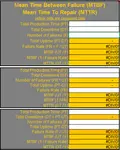
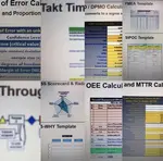
Six Sigma Templates, Tables, and Calculators. MTBF, MTTR, A3, EOQ, 5S, 5 WHY, DPMO, FMEA, SIPOC, RTY, DMAIC Contract, OEE, Value Stream Map, Pugh Matrix -
Six Sigma, Six Sigma Training, Courses, Calculators, Certification
Aug 15, 21 10:27 PM
 One site with the most common Six Sigma material, videos, examples, calculators, courses, and certification.

Site Membership
LEARN MORE
Six Sigma
Templates, Tables & Calculators
Six Sigma Slides
Green Belt Program (1,000+ Slides)
Basic Statistics
Cost of Quality
SPC
Control Charts
Process Mapping
Capability Studies
MSA
SIPOC
Cause & Effect Matrix
FMEA
Multivariate Analysis
Central Limit Theorem
Confidence Intervals
Hypothesis Testing
Normality
T Tests
1-Way ANOVA
Chi-Square
Correlation
Regression
Control Plan
Kaizen
MTBF and MTTR
Project Pitfalls
Error Proofing
Z Scores
OEE
Takt Time
Line Balancing
Yield Metrics
Sampling Methods
Data Classification
Practice Exam
... and more