t-distribution (t-tests)

The various t-tests are applied during the ANALYZE and CONTROL phase. You should be very familiar with these test and able to explain the results.

William Sealy Gosset is credited with first publishing the data of the test statistic and became known as the Student's t-distribution. This is used to estimate the parameters of a population when the sample size is small.

The t-test is generally used when:

• Sample sizes less than 30 (n<30)
• Standard deviation is UNKNOWN 

The t-distribution bell curve gets flatter as the Degrees of Freedom (dF) decrease. Looking at it from the other perspective, as the dF increases, the number of samples (n) must be increasing thus the sample is becoming more representative of the population and the sample statistics approach the population parameters.

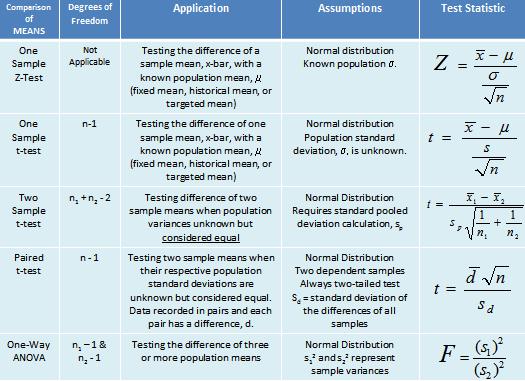
As these values come closer to one another the "z" calculation and "t" calculation get closer and closer to same value. The table below explains each test in more detail.

---

Hypothesis Testing

T-tests are very commonly used in Six Sigma for evaluating means (μ) of one or two populations. You can use a t-test for determining if:

• One mean from random sample is different than a target value, a known mean, or a historical mean.
• Two group means are different.
• Paired means are different. 

The word different could be greater than, less than, or a certain value different than a target value. You can run statistical test in software usually be easily configuring the parameters to look for certain types of differences as were just mentioned. 

For example, instead of just testing to see if one group mean is different than another, you can test to see if one group is a greater than the other and by a certain amount. You can get more information by adding more specific criteria to your test.

Before running a test, visualize your data to get a better understanding of the projected outcome of expected result. Using tools such as Box Plot can provide a wealth of information.

Also, if the confidence interval contains the value of zero then insufficient evidence exist to suggest their is a statistical difference between the null and alternative hypotheses and accept the null.

---

---

One Sample t-test

This test compares a sample to a known population mean, historical mean, or targeted mean. The population standard deviation is unknown and the data must satisfy normality assumptions.

Given:
n = sample size
Degrees of freedom (dF) = n-1

Most statistical software will allow a variety of options to be examined from how large a sample must be to detect a certain size difference given a desired level of Power (= 1 - Beta Risk). You can also select various levels of Significance or Alpha Risk.

For a given difference that you are interested in, the amount of samples required increases if you want to reduce beta risk (which seems logical). However, gathering more samples has a cost and that is the job of the GB/BB to balance getting the most info to get more Power and highest Confidence Level without too much cost or tying up too many resources.

Example of One Sample t-test

The following example shows the step by step analysis of a One Sample t-test. The example uses a sample size of 51 so usually the z-test would be used but the result will be very similar.

The sample standard deviation would be the population standard deviation since the sample size is large enough (>30). Also the degrees of freedom (dF) are not applicable. The point to take away are the steps applied and the interpretation of the final results.

---

Example of a Two Sample t-test

This test is used when comparing the means of:

1) Two random independent samples are drawn, n₁ and n₂
2) Each population exhibit normal distribution
3) Equal standard deviations assumed for each population

The degrees of freedom (dF*) = n₁ + n₂ - 2

*There is another more complicated formula for dF if the two population standard deviation are NOT assumed to be equal. 

Example:

The overall length of a sample of a part running on two different machines is being evaluated. The hypothesis test is to determine if there is a difference between the overall lengths of the parts made of the two machines using 95% level of confidence.

Our sample size has already been confirmed that we need 20 samples (from each machine) to provide 80% Power.

Machine 1 (call this the OLD machine):

Sample Size: 25 parts
Mean: 24.12 mm
Sample standard deviation: 5.52 mm

Machine 2 (call this the NEW machine):

Sample Size: 20 parts
Mean: 19.15 mm
Sample standard deviation: 6.51 mm

dF = n₁ + n₂ - 2 = 25+20-2 = 43
Alpha-risk = 1-CI = 1-0.95 = 0.05 (95% level of significance)

Establish the hypothesis test:

Null Hypothesis (H_O): Mean₁ = Mean₂
Alternative Hypothesis (H_A): Mean₁ does not equal Mean₂

This is two-tailed example since the direction (shorter or longer) is not relevant. All that is relevant is if there is a statistical difference or not.

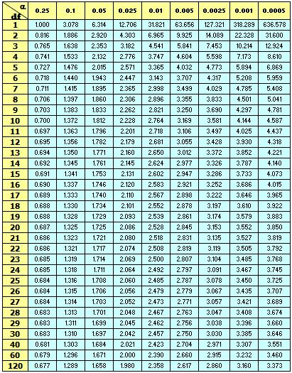
Now, determine the range for which t-statistic and any values outside these ranges will result in rejecting the null and inferring the alternative hypothesis. Using the t-table below notice that:

-t(0.975) to t(0.975) with 43 dF equals a range of about -2.02 to 2.02.

If the calculated t-value from our example falls within this range then accept the null hypothesis.

NOTE: The table below is a one-tailed table so use the column 0.025 that corresponds to 40 dF and include both the positive and negative value.

43 dF isn't exactly shown in this table but you can figure out that the value will be near 2.02 since it is trending downward from 40 dF to 60 dF. You could do a mathematical interpolation but it could be a waste of time since the t-statistic probably won't be that close to the this t-table value of 2.02. 

Interpreting the results

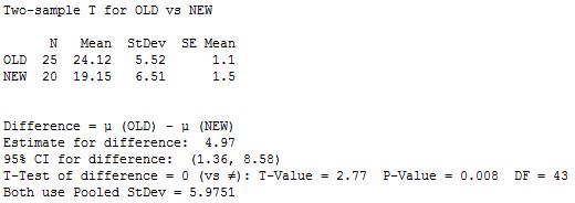
The display above is a common output of running a Two Sample t-test.

In this example, both samples exhibit normal behavior and it was assumed that the variance are equal and the dF = 20 + 25 - 2 - 43 The hypothesized difference is 0.

Assumed equal variances so the pooled standard deviation is used. The estimate for the difference is the difference from the OLD to NEW mean. With an alpha-risk of 5% (or CL of 95%) the difference will be between 1.36 and 8.58.

The p-value is 0.008 which is much less than 0.05, therefore reject the H_O and infer the H_A that there is a statistical difference in the means of the two machines. 

When to assume EQUAL VARIANCES or UNEQUAL VARIANCES?

The answer isn't as straightforward as one might hope. For the sake of keeping it simple and understanding there may be exceptions, generally you can assume equal variances unless:

• comparing vastly different sample sizes
• knowingly have unequal variances
• used the F-test and you detemine that the variance of the samples are unequal. 

Some statisticians suggest taking the more care and conservative approach and assume unequal variances all the time. This method covers for the worst case scenairo that the variance are truly unequal and only forgoes a minute amount of statistical power. In other words, sacrifice a little power to protect for the worst case.  

---

Paired t test

Comparing the difference between two paired sample means (each with the same number of samples) from two normal distributions.

ASSUMPTIONS:

• The values must be obtained from the same subject (machine, person) each time.
• The values from the “differences” must be normal
• Values must be independent (i.e. the samples don’t impact each others measurements)

Use this test when analyzing the samples of a BEFORE and AFTER situation and the number of samples must be the same. Also referred to as "pre-post" test and consist of two measurements taken on the same subjects such as machines, people, or process.

This option is selected to test the hypothesis of no difference between two variables. The data may consist of two measurements taken on the same machine (or subject) or one before and after measurement taken on a matched pair of subjects.

For example, if the Six Sigma team has implemented improvements from the IMPROVE phase they are expecting a favorable change to the outputs (Y). If the improvements had no effect the average difference between the measurements is equal to 0 and the null hypothesis is inferred.

If the team did a good job making improvements to address the critical inputs (X's) to the problem (Y's) that were causing the variation (and/or to shift the mean in unfavorable direction) then their should be a statistical difference and the alternative hypothesis should be inferred.

dF = n - 1

The "Sd" is the standard deviation of the difference in all of the samples. The data is recorded in pairs and each pair of data has a difference, d.

Another application may be to measure the weight or cholesterol levels of a group of people that are given a certain diet over a period of time.

The before data of each person (weight or cholesterol levels) are recorded to serve as the basis for the null hypothesis.

With the other variables controlled and maintained consistent for all people for the duration of the study, then the after measurements are taken.

The null hypothesis infers that there is not a significant difference in the weights (or cholesterol levels) of the patients.

H_O: Mean_before = Mean_after

H_A: Mean_before ≠ Mean_after

Again, this test assumes the data set are normally distributed and continuous.

Practice Certification Questions

1) Find the Degrees of Freedom (dF) if running a paired t-test with samples of 15.

A) 15

B) 13

C) 14

D) 29

The answer is dF = n-1 = 15-1 = 14

This value is used in calculating each sample standard deviation and the Standard Error of the Mean (in the denominator) for each sample.

2) If sample sizes are 13 (n=13) and the alpha-risk is chosen to be 0.05, what is the critical t-value for a two tailed paired-t test?

The dF = 12 and since it is two-tailed you look at the column below that is 0.025 (the alpha-risk divided by two).

t_critical = 2.179

See the table below and see that a dF of 12 and alpha-risk of 0.025 = 2.179

3) If the sample size is 26 for each of two pairs of data, the average of the differences of paired values (dbar) is 0.77, and the standard deviation of the values of the differences is 3.43, what is the t-statistic?

For paired t-test (assuming the values of differences has been confirmed to be normal).

N-1= n, so n = 25

t = (dbar) * √n / S_d

t = (0.77 * √25) / 3.43

t = 3.85 / 3.43

t = 1.12

---

t-distribution table

---

t test in Excel

The formula returns the probability (p-value) associated with the Student's t-test.

T.Test (array1, array2, tails, type)

Each array (or data set) must have the same number of data points.

The "tails" represents the number of distribution tails to return:

1 = one-tailed distribution

2 = two-tailed distribution

The "type" represent the type of t-test. 

1= paired

2 = two sample equal variance

3 = two sample unequal variance

---

Z test

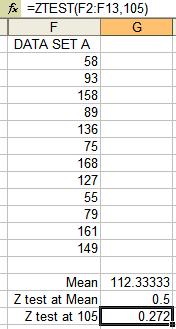
The Z test uses a set of data and test a point of interest. An example is shown below using Excel. This function returns the one-tailed probability.

The sigma value is optional. Use the population standard deviation if it is known. If not, the test defaults to the sample standard deviation.

Running the Z test at the mean of the data set returns a value of 0.5, or 50%.

EXAMPLE:

Recall the sample sizes are generally >30 (the snapshot below uses fewer only to illustrate the data and formula within Excel within a reasonable amount of space) and there is a known population standard deviation. 

The data below uses a point of interest for the hypothesized population mean of 105.

This corresponds to a Z test value of 0.272 indicating that there is a 27.2% chance that 105 is greater than the average of actual data set assuming data set meets normality assumptions.

The Z test (as shown in the example below) value represents the probability that the sample mean is greater than the actual value from the data set when the underlying population mean is μ0.

The Z-test value IS NOT the same as a z-score.

The z-score involves the Voice of the Customer and the USL, LSL specification limits.

Six Sigma projects should have a baseline z-score after the Measure phase is completed and before moving into Analyze. The final Z-score is also calculated after the Improve phase and the Control phase is about instituting actions to maintain the gains.

There other metrics such as RTY, NY, DPMO, PPM, RPN, can be used in Six Sigma projects as the Big "Y" but usually they can be converted to a z-score (except RPN which is used within the FMEA for risk analysis of failure modes).

---

Confidence Interval Formula

---

T-test or Z-test?

---

Example Certification Questions

1) A Green Belt wants to evaluate the output of a process before and after a set of changes were made to increase the productivity. The data acquired meets the assumption of normality. Which hypothesis test is best suited to determine if the changes actually improved the productivity?

A) Paired-t test

B) Two sample t test

C) ANOVA

D) F-test

Answer: A

2) If a Black Belt wants to test if a supplier can produce a batch of parts in less than 5 business days, which t test would be used?

A) One sample t test

B) Two sample t test

C) Paired sample t test

Answer: A, and a one-tailed test. 

3) If a Black Belt wants to test the productivity of two machines in terms of pieces/hour and determine whether there is a difference, which test should be used?

A) One sample t test

B) Two sample t test

C) Paired sample t test

Answer: B, and a two-tailed test. 

Want more? Test your knowledge with over 180 practice questions. 

---

Return to BASIC STATISTICS

Return to the ANALYZE phase

Templates, Tables, and Calculators

Search for Six Sigma related jobs

Return to the Six-Sigma-Material Home Page