|

 content.")

Data Collection
Description:
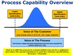
Documented procedure for standardized and efficient data collection. A process for collecting data that will be used to describe the Voice of the Process (VOP).
Objective:
Ensure the data collection is complete, realistic, and practical. Often times, data collection can be costly and encounter resistance by those involved. Strive to minimize the costs and impact to those involved while obtaining as much accurate data in reasonable amount of time.
Data Collection Process
STEP 1: When setting up the collection system it is important to collect data only once and minimize the burden on the operators, team, and the GB/BB. Ensure to capture all the families of variation (FOV) that should be analyzed or relevant.
Create a Families of Variation (FOV) diagram.
Think about all the factors that contribute to the process performance (mean and variance).

The entire amount of variation found in a set of data can be broken down
to the variation from the Process + the variation from the Measurement
System, which should be calculated from the MSA.
If:
The % Study Variation in the MSA was found to be X, the Process Variation = 1 - X.
A FOV diagram evaluates the sources of Process Variation. These sources include families such as:
- Part-Part
- Shift-Shift
- Operator-Operator
- Machine-Machine
- Form-Form
- Facility-Facility
- Tool-Tool
- Date/Time (always important to collect the time and date)
You must collect at least data from every family of variation. Too much information is not a bad thing if its easily and readily available.
Another possibility is shown
below. Each one of the families will contribute to the overall process
performance. The combination (not necessarily the sum) of all their
variances represents the overall process variance. These are all "short"
term sources that make up the "long" term variation.

STEP 2: Complete a simple but comprehensive form that elaborates on the
data and collection plan. There is a free template below. Modify it to fit your project and FOV's.
This may later be used as an attachment used
in the Control Plan when handing-off the project to the Process Owner.
Other items in addition to the FOV tree when completing the Data Collection Plan are:
Items to include in the Data Collection Plan:
- What is the question the team is trying to answer?
- What metrics are being measured?
- What is the best sampling strategy?
- Sample size (may need visit Power and Sample Size) needed
- Where observations are collected?
- How the observations are measured, what devices and units?
- How the observations are recorded?
- Do I have rational subgroups (read below)?
- Recording frequency
- Data Classification
- Pictures, videos, screenshots, macros, reference documents
Review the types of data and necessary sample sizes (observations) needed to create control charts and hypothesis testing coming up later in the MEASURE and ANALYZE phases.
Meeting or exceeding the minimum (without being too costly) can lead to better analysis and stronger decision making.
STEP 3: Collect the data carefully.
As you can read below, continuous data is more informative than attribute data. However, it may not be possible or practical to get continuous data for each FOV.
Free Data Collection Template
 |
Click here to download a free Data Collection Plan template with a few examples. |
Discussion
Data collected through automated methods often have the most accuracy and consistency (however can be consistency wrong too). Even as simple as they seem to collect data, it is important to
clearly identify the source, system, menus, files, folders, etc. that
the information lies within. Any macros and adjustments and such should
be written out with clear step-by-step instructions.
Automated systems can be timely and expensive to install. However, improving a data collection system can be a very
successful part of the project improvement process in itself. This can become a project in a project so be careful to avoid one of the most common Project Pitfalls called Paralysis from Analysis.
Manual
methods require more instructions and training. Minimize the amount of
people involved to reduce risk of introducing variation. The higher
level of instruction and detail provided to the data collectors and
appraisers (those collecting the measurements) will reduce the variation
component contributed from the measurement system. This amount of error
will be quantified and examine in the Gage R&R.
This is
usually inexpensive to put in place and should be suited to fit exactly
to what is needed. However, it can be costly in terms of being labor
intensive, prone to recording errors and troubleshooting suspicious
data.
Adding videotape and recordings are excellent ways to
capture data and have the advantage of replay. This helps remove uncertainty in
what actually occurred.
Attribute Data Collection
Attribute data are fixed gauges that provide limited information but can be cheaper and quicker devices to obtain a decision that meets the Voice of the Customer. They are used to make decisions such as:
- Pass / Fail
- Go / No-go
- In / Out
- Hot / Cold
- Good / Bad
...but
they don't tell how good or how bad the measurement is relative to
specification limits. Each decision is given the same weight but some 'GO' decisions may be actually better than others so that is where more
discrimination (or resolution) in the measurement system can help and
that comes with variable data.
Types of attribute measurement devices are:
- Plug Gauges
- Gage Blocks
- Flush Pin
- Bench Gauges
- Sight Gauges
- Positional Gauges
- Thread Gauges
- Limit Length Gauges
Variable Data Collection
These measurement devices provide more information that attribute gauges and should be used to measure critical characteristics at a minimum. They provide a measured dimension. Types of variable measurement devices are:
- Hardness Tester (Mohs, File, Sonodur, Rockwell, Vickers, etc.)
- Calipers
- Micrometers
- Tensile Tester
- Ruler or Tape Measure
- Bore Gauges
- Indicator Gauges
- Height Gauges
- Amp Meter
- Ohm Meter
- Air gauging
Rational Subgrouping
Why is rational subgrouping important?
These represent small samples within the population that are obtained at similar settings (inputs or condition) over short period of time. In other words, instead of getting one data point on a short-term setting, obtain 4-5 points and get a subgroup at that same setting and then move onto the next. This helps estimate the natural and common cause variation within the process.
Individual data (I-MR) is acceptable to measure control; however, it usually means that more data points (longer period of time) are necessary to ensure that all the true process variation is captured. The subgroup size = 1 when using I-MR charts.
Sometimes this can be purposely controlled and other times you may have to recognize it within data. Often times, a Six Sigma Project Manager will be given some data with no idea on how it was collected.
The data table below shows that 50 samples were collected and measured within 10 subgroups of 5 measurements each. The appraiser took five measurements at a particular moment (same tool, same operator, same machine, same short term time frame) and recorded measurements of the diameter of each part.
This extra data (yes, it is more work and time) allows much stronger capability analysis rather than just collecting 10 data points, one reading from each part where a subgroup size = 1.
The x-bar value for each subgroup is the average reading of each subgroup and the range is easily calculated for each subgroup as the difference between the maximum and minimum value within each subgroup.
 Rational Subgrouping at Six-Sigma-Material.com
From here you can use the data to manually create x-bar control charts and calculate control limits. The average of the averages is 27.9083.
If there was a known standard value for the diameter, then the Gauge Bias can also be determined by taking 27.9083 minus the Standard Value. Assume the Standard (Reference) is 27.9050 then:
Gauge Bias = 27.9083 - 27.9050 = 0.0033 (this value is used when assessing gauge bias during a Stability review as part of MSA)
Another Example: Here we discover subgroups within the data (a good thing).
A Black Belt (BB) is provided data (different data than used above) from the team and begins to assess control. Without understanding the data and how it was collected, the BB generates the following Individuals chart indicating the Miles Per Gallon (MPG) of a vehicle from 23 observations.

The visual representation makes it clearer that there are likely subgroups within the data. The control chart appears to be out of control with a lot of special cause variation but there is likely a good explanation.
The BB talks to the team and learns that the MPG were gathered at different slopes of terrain. The higher MPG readings were achieved on downhill slopes and vice versa. The data is more appropriately shown below.

This shows each subgroup being in control. There were short term shifts in the inputs or conditions. Assessing normality or capability on the entire group of data is not meaningful since the inputs were purposely changed to gather data on different conditions. Therefore, this is not a "naturally" occurring process. There is going to be an appearance of "special cause" variation when in fact it is not.
Try to break down the data into the subgroups and analyze the data for normality and capability of each subgroup.
The next important measurement for someone looking at this data could be to understand that incline and decline measurements for each subgroup and determine the correlation between MPG and angle of incline or decline.
The point is to look for subgroups within the data and this provide a plausible explanation of what initially appears to be special cause variation.
Data Coding
Data Coding is a method of improving the efficiency of data entry by changing the WITHOUT reducing the accuracy and precision of the data.
In other words, keep the integrity of the data but improve the speed of data collection.
Sometimes people try to write too much data on a sheet and it becomes unreadable and/or all the digits are unnecessary.
Sometimes too much data resolution (or discrimination) does more harm than good. You always want to get enough discrimination but too much can be time consuming to collect.
Summary
Measurements are the basis for everything in quality systems for two primary reasons:
- To make an assessment or decision
- To measure process improvement or lack thereof
Without
measurement there cannot be objective proof or statistical evidence of
process control, shift, or improvement. It's critical to
get the most informative data that is practical and time
permitting.
This data is required to understand the measurement system variation (done via MSA) and the process variation.
Once
the MSA is concluded (and hopefully passed) the remaining variation is
due to the process. The Six Sigma team should focus on reducing and controlling the process variation. However, sometimes fixing the measurement system itself can be a Six Sigma
project if the potential is significant and the current system is so
poor that it prohibits process capability analysis.
Gauges
require care and regular calibration to ensure the tolerances are
maintained and ensure the amount of variation they are contributing to
the total variation is constant and not changing or that could affect
decisions being made about the process variation (that are not actually
occurring since the variation changes are stemming from the measurement
devices).
Some gauges require special storage or have standard
operating procedures. Any time there is suspected damage
or a unique event that will use a device to a higher than usual degree, then a calibration should be done.
Such as in a physical inventory event, all weigh scales should be calibrated prior to the event. All personnel should be trained on the same procedure and understand how the scales work.
Spend the time up front to remove the sources of variation and capture the most meaningful data.
GOAL:
The goal is to have the sources of variation come from only the process and not the measurement system. Strive to capture the data using rational subgrouping across entire spectrum of sources of process variability.
Templates, Tables, and Calculators
Search for active Six Sigma related job openings
Return to Six-Sigma-Material Home Page
Recent Articles
-
Process Capability Indices
Oct 18, 21 09:32 AM
 Determing the process capability indices, Pp, Ppk, Cp, Cpk, Cpm
 -
Six Sigma Calculator, Statistics Tables, and Six Sigma Templates
Sep 14, 21 09:19 AM
 Six Sigma Calculators, Statistics Tables, and Six Sigma Templates to make your job easier as a Six Sigma Project Manager
 -
Six Sigma Templates, Statistics Tables, and Six Sigma Calculators
Aug 16, 21 01:25 PM
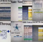
Six Sigma Templates, Tables, and Calculators. MTBF, MTTR, A3, EOQ, 5S, 5 WHY, DPMO, FMEA, SIPOC, RTY, DMAIC Contract, OEE, Value Stream Map, Pugh Matrix
Recent Articles
-
Process Capability Indices
Oct 18, 21 09:32 AM
Determing the process capability indices, Pp, Ppk, Cp, Cpk, Cpm -
Six Sigma Calculator, Statistics Tables, and Six Sigma Templates
Sep 14, 21 09:19 AM
Six Sigma Calculators, Statistics Tables, and Six Sigma Templates to make your job easier as a Six Sigma Project Manager -
Six Sigma Templates, Statistics Tables, and Six Sigma Calculators
Aug 16, 21 01:25 PM
Six Sigma Templates, Tables, and Calculators. MTBF, MTTR, A3, EOQ, 5S, 5 WHY, DPMO, FMEA, SIPOC, RTY, DMAIC Contract, OEE, Value Stream Map, Pugh Matrix -
Six Sigma, Six Sigma Training, Courses, Calculators, Certification
Aug 15, 21 10:27 PM
 One site with the most common Six Sigma material, videos, examples, calculators, courses, and certification.

Site Membership
LEARN MORE
Six Sigma
Templates, Tables & Calculators
Six Sigma Slides
Green Belt Program (1,000+ Slides)
Basic Statistics
Cost of Quality
SPC
Control Charts
Process Mapping
Capability Studies
MSA
SIPOC
Cause & Effect Matrix
FMEA
Multivariate Analysis
Central Limit Theorem
Confidence Intervals
Hypothesis Testing
Normality
T Tests
1-Way ANOVA
Chi-Square
Correlation
Regression
Control Plan
Kaizen
MTBF and MTTR
Project Pitfalls
Error Proofing
Z Scores
OEE
Takt Time
Line Balancing
Yield Metrics
Sampling Methods
Data Classification
Practice Exam
... and more