|

 content.")
Economic Order Quantity (EOQ)
Objective:
Determine the optimum level of ordering frequency and amount of units. The amount of units is called the Economic Order Quantity (EOQ) or Economic Lot Size (ELS).
Units may be pieces, items, each, widgets, etc. It is calculated specific to each product (unless all the variables happen to be the same for more than one product).
The proper use of EOQ by product is essential for an effective JIT program. There is one basic commonly accepted formula but it relies on accurate inputs and relates more for buying and single-step manufacturing.
The formula is simple. However the inputs can be challenging to get right.....and they change over time. Since these variable change, EOQ calculations must be constantly reviewed and updated. Some simple software with inputs entered into on a regular basis is all that is needed.
. Also known as the Economic Lot Size (ELS).")
As with many formulas there are key assumptions and limitations. For the simple EOQ formula shown above we assign the following:
EOQ = Economic Order Quantity (or ELS for single-step manufacturing).
- F = Costs to execute an Order or Acquisition Costs (Fixed Costs per EOQ Batch)
- I = Inventory Carrying Rate (expressed as %)
- C = Cost per Unit ($/unit)
- H = Holding (Carrying) Costs per Unit per Unit of Time* = I * C
- D = Demand per Unit of Time* (assumed constant rate of demand)
*The Unit of Time for H and D must be the same (year, month, etc.)
With the fixed demand rate, shortages can be avoided by replenishing inventory each time the inventory level drops to zero and this also will minimize the holding cost.
Assumptions:
The following are assumed:
- Known constant demand rate of a units per unit time. Such as 4,923 pieces per month or 59,076 pieces per year. In other words, the customer pulls at a constant demand rate.
- Assumed C is the same for any quantity purchased. This means there is not a minimum order quantity or quantity discount option.
- The EOQ to replenish inventory arrives on time and all at once when the inventory reaches zero. Lead time is constant.
- No planned shortages and inventory are replenished as needed. In this case, we assume that holding zero inventory is not allowed for any period of time. Obviously some businesses can take the risk but we will keep things simple.
- The unit cost per piece (I) to purchase or produce cannot be zero.
- Carrying cost cannot be zero to use this formula. If it is, which it could be in reality, then your EOQ is as many as you can sell immediately. This could be infinite.
CAUTION:
The EOQ described here is similar to an ELS for one production operation. However, it is different that the Economic Lot Size (ELS) to produce when a product goes through a manufacturing sequence of more than one process (that is described later).
For most businesses, the correct EOQ should also prevent running out and risking the loss of customer revenue by not have available inventory to sell. The correct EOQ minimizes the company costs while maintaining just the right amount of inventory to meet customer demand.
Since there is variation in all the inputs, when determining the EOQ it is a good idea to model scenarios using the same formula but entering more extreme inputs to get a
- WORST case - an unlike case but using plausible numbers that could happen which would provide you a higher total costs value.
- BEST case - an unlikely case but using plausible numbers that could happen to minimize your total costs
- IDEAL case - a most likely scenario for your total costs.
Think of it as a Confidence Interval.
Determine a lower and upper end so you can plan to both scenarios with the expectation to fall somewhere between the two boundaries.
An EOQ for one business, or one factory within a business, may vary even if they produce or purchase the same exact product. Each location has a unique fixed costs structure and may have a unique carrying costs of inventory.
What you need to know:
The Unit Cost per Item (C) to buy at various quantities. Maybe it's one price regardless of volume. That is the simplest case but often there may be quantity breaks, which usually means a quantity discount if more are purchased at once. Purchasing more at once may give you a better unit price but normally means more carrying costs over the long run since that inventory is likely to sit for a period of time. This period of time may be near zero seconds or several days or years.
Inventory Holding (or Carrying) Costs (H) or as a % of the Unit Cost per Item (I). This value normally comes from the Finance Department. Also referred to as variable costs. When you have cash tied up in goods that are sitting on the shelf waiting to be sold, that costs money. Money that could be used for other investments, pay down interest, pay for storage fees, insurance, people to watch the site, taxes, etc.
That is why this may also be the opportunity costs where if you didn't spend the money carrying the inventory, how much money could be made if that money was used somewhere else? In some cases. the carrying costs may be zero. If you're fortunate enough to have an e-commerce site where you aren't responsible for inventory or another arrangement where the entire EOQ batch ships at once (and you get paid for it all at once).
If you get H as a value from Finance, then you don't need I and C.
Fixed Cost to Execute an Order of Units (F): Another value normally provided by the Finance Department This is also referred to as the Acquisition Cost per Order. How much does it cost to execute and order from quote, PO, supplier management, freight, handling, admin costs, etc.
Annual Volume or Demand (D) - be careful with this value. This is a Number of Pieces (units, items) over a Unit of Time. Usually it is Pieces / Year. Most importantly the unit of time must be consistent throughout the EOQ formula if you decide to use a unit of time other than year. Think about how much is FIRM (i.e. are you able to sell) and how much is a FORECAST which may not sell. Or the forecast could be too low and thus your actual volume may end up being more. This results in determining an EOQ that is lower than optimal.

Perfect World - Reorder Point
Remember from earlier, to keep the example simple, the Lead Time (LT) is assumed constant. The LT is amount of time between issuing the order and its receipt (and able to ship to the customer). The inventory level at which the order is placed is called the Reorder Point (RP)
If the LT is always the same, the RP equals the lead time * demand rate. The key is to keep the "unit of time' consistent. See the example below
RP = Reorder Point = LT * D
Example:
If the lead time to buy an EOQ of 100 pieces is 50 calendar days and the annual demand is 500 pieces per year, calculate the RP.
First of all, convert 500 pieces/year to pieces/calendar day. This is 1.37 pieces/day.
RP = LT * D = 50 days * 1.37 pieces/day = 68.5 pcs (round up to 69 pieces)
In a perfect world, the point at which to issue a new order for 100 pieces is when the inventory is depleted to a level of 69 pieces.
69 pieces will last just over 50 calendar days if the customer demand is 1.37 pieces/day. This is a bold assumption since customer demand is almost never a constant rate. You may choose to take a little risk to buffer for some variation in the customer demand rate and choose 70 or 75 pieces are a RP.
For more information on accounting for Buffer and Safety stock, see our Kanban module.
EOQ Calculation Example
Determine the EOQ given the following information:
F = the fixed cost to execute an order costs $40
I = Finance determines the carrying % to be 20%
C = the cost per unit is $1.50/each to purchase from the supplier
H = Annual Holding (Carrying) Costs = I * C = $1.50 * 0.20 = $0.30/each
D = Annual demand is 10,000 pieces

EOQ Calculator
Try it for yourself. Plug in your numbers below.
The calculator above is a basic version of our advanced version that includes an interactive data readout with a dynamic graph to help illustrate the impact of various EOQ's. It allows you to quickly model various inputs and understand a range for your EOQ.
Shown below is the example above. Enter any numbers and you'll see the impact to all the outputs and most importantly, the Total Annual Costs.
Visit Templates, Tables, and Calculators to see this one and several others.
 to model various scenarios. This calculator is available at https://www.six-sigma-material.com/Six-Sigma-Templates.html")

%20is%20a%20fairly%20simple%20equation%20but%20making%20the%20correct%20assumptions%20and%20keeping%20those%20assumption%20accurate%20over%20time%2C%20is%20the%20challenge.)
Notice above, the lowest point in the 'Annual Costs' line is the EOQ which is 1,633 pieces in this case. The 'Annual Costs' is $490 at this EOQ when ordered 6 times/year at even time intervals (perfect world case).
Keep in mind the 'Total Unit Costs' is the same of all EOQ's since it is just the Annual Demand of pieces * the Unit Cost per Piece.
EOQ Assumptions/Risks
The following are risks and considerations when determining the EOQ (ELS):
- The annual volume (customer pull rate) may change over time. For instance, a 12 month forward plan as of today may appear to be X units. However, a month from now the 12 month forward plan may not be X units - it could be more or less. Therefore it's important to understand if the volume is dynamic.....and it usually is. Therefore, it is important to recalculate the EOQ periodically and try to level load (i.e. produce a consistent amount each time) around that EOQ. Another point to observe is the customer is likely to pull orders from your inventory on a variable pattern. This variation should be measured and accounted for in the variation. Any variation means that the EOQ needs to be inflated to cover that risk unless you can afford to run out of stock.
- Does the item have a shelf life? If the product can only sit in inventory for a limited time, you'll need to make sure that the EOQ isn't so large that the inventory is at risks of sitting beyond its shelf life.
- Are there external factors that add risk to your supply chain? such as the risk of geopolitical events like tariffs or natural disasters such as hurricanes. You may need to buy or produce more or less early or delay, depending on the information.
- Fixed Cost to execute an order can change. Obviously, every variable can change. This is normally provided by Finance. Ensure to check in periodically to get this value updated.
- Holding Costs and opportunity costs can change. Same as above. Try to minimize your carrying costs through smaller batches, less variation, or changing the customer buying policy.
- Can your business allow planned shortages without losing money? If so, a greater risk can be taken on the level of inventory maintained. The formula gets more complicated and is not discussed here.
- The Cost Per Unit can change depending on the quote. Perhaps the quote has an expiration date where that could result in a change in price. Or there may be a quantity break where a lower price could apply with a higher volume of purchase. Perhaps you have dual sourced the item to have a back-up source but the prices are different. In that case you may calculate a weighted-average cost per unit and use that value for C
The EOQ (or ELS) value is easy to calculate.....once you have the numbers. However, the assumptions are difficult. The EOQ (or ELS) value is only as valid as its inputs. At some point, assumptions and agreements need to be made on the inputs.
Garbage IN - Garbage OUT. Spend the time to get the inputs correct and challenge the assumptions.
Observations
Notice the inputs in the numerator and denominator: A large or small EOQ is neither good or bad. It depends on your situation and the impact each direction has on your inputs.
If F increases (D and H are constant), EOQ increases
Longer set-up times and fixed costs drive up batch size. Maybe a SMED event will reduce set-up times thus reducing EOQ.
If F decreases (D and H are constant), EOQ decreases
This results in more set-ups (or purchase) but they are quicker or the cost to execute a purchase has been reduced. Maybe you issue a Blanket PO instead of a discrete PO each time. Lower EOQ means less carrying costs. And if there is a quality issue, there may be less product to quarantine or scrap.
If D increases (F and H are constant), EOQ increases
which should be a good thing to have more sales and hopefully more profit. You may use this as an opportunity to negotiate a higher volume discount if buying a product.
If D decreases (F and H are constant), EOQ decreases
Sales are lower, profit is lower and you may face inflation due to lower volume. The contribution margin is lower per piece. This isn't the ideal way to reduce EOQ (or ELS).
If I increases (C, D and F are constant), EOQ decreases
If the costs to carry inventory increases (lease increased, insurance, labor, taxes, etc.), the EOQ drops to recommended carrying less product at a given time.
If I decreases (C, D and F are constant), EOQ increases
The closer I gets to $0, the more and more you can put on the shelf and carry since it is getting close to free to carry. Putting anything on a "shelf" isn't likely to be free even if it's for a few minutes. If you have a drop-ship business without any inventory liability then your EOQ is as high as you can sell. This could be infinite.
If C increases (D, I, and F are constant), EOQ decreases
If the purchase cost per unit or the variable production costs increase, then EOQ decreases. Higher costs to manufacture or purchase means you don't want to carry as much on the shelf at any given time. That ties up cash sitting on the shelf waiting (and hoping to be sold).
If C decreases (D, I, and F are constant), EOQ increases
If the purchase cost per unit or the variable production costs decrease, then you can afford to buy more at once to carry. Try to negotiate a lower cost and then you can commit to buy more per order to the supplier. Could be a win-win.
Remember, I * C = H. This means that I could go down, but C goes up to the point where H increases and thus the EOQ decreases or vice versa.
ELS for multiple manufacturing operations
If you're manufacturing a product that goes through one step, the Economic Lot Size (ELS) is generally applicable.
An ELS for one operation may not be ideal for a different operation(s). It's important to build an ELS that optimizes the entire value-stream rather than one (or two operations).
There isn't a formula that suits every situation. It can be a complex math problem which is solvable but needs input from several departments to get it accurate.
Let's discuss the variables for calculating ELS for multiple operations:
Fixed Cost per Order - would include costs such as Set-Up Time, etc. but it calculated for each process step. If the Set-Up time for one process is much greater than another, it is likely to drive up the ELS for the entire value stream.
Unit Cost to Produce - instead of Unit Cost to Purchase. Calculate the variable costs to produce the item at each process step. Such as tools, oil, MRO, utilities, etc. This can be difficult especially when there are some semi-variable costs. Don't forget to include direct and indirect costs.
It gets more complicated if the manufacturing process also involves outside operations. Some external suppliers (or processors) may require a minimum batch size or there is a premium to pay. They may also have other irregular fees such as testing fees, certification fees, or monthly surcharges. All these costs need to be part of the conversation when you're determining the ELS for that process step.
Consider freight, handling, insurance, and all the costs involved. It always ideal to come up with a lower ELS than expected but that only creates problems down the road if it isn't accurate.
Consider the container size or the container of the inputs. For example, if you are stamping it may be optimal to run a full coil and use that as the ELS, if new coil replenishment takes a long time. Perhaps this can be done as an external set-up function at another time.
Or a racking device, perhaps a full rack is the best ELS instead of risking running a partially full rack.
Calculate the ELS for each process step. This could generate some surprises and more value-added ideas. Next, discuss Lot Integrity.
Is Lot Integrity required?
In some business, you must maintain Lot integrity, in other words you cannot mix lots (or batches). Once you start a batch it can't be mixed with others in downstream operations. It can be broken up to smaller lots with traceability, but it cannot grow after the first operation. This makes it even more challenging.
An ELS that makes sense for one operation will not be optimal for other(s). You'll have to determine with ELS of all the ELSs' offer the best overall financial performance.
If your business can mix lots and batches, then try to produce the ELS for each operation when the Reorder Point is reached. That way you get the optimal financial advantage from each operation. But this isn't always practical.
Summary
If you're manufacturing using several processes to make an item, the costs per unit are almost constantly changing.
Variable costs from tooling, labor, utilities, freight, MRO, are examples that change regularly. Some assumption needs to be made to start the ELS calculation. Periodically all the variables should be updated to reflect a new ELS.
The Lead Time is from the start of the first operation to the point the product is saleable. This includes all the non-value added and value added steps (handling, moving, waiting, shipping, testing, etc.). This drives up the Reorder Point.
This is another reason the Lean Manufacturing tools of 7-Wastes, Process Mapping, Spaghetti Diagram, and Value Stream Mapping, Takt TIme/Load Balancing are valuable.
By merely going through this exercise with the Six Sigma/Lean Team, you will almost certainly generate some passionate discussion on new ideas or paradigm challenges. This is exactly what you want as a Green Belt/Black Belt.
Recent Articles
-
Process Capability Indices
Oct 18, 21 09:32 AM
 Determing the process capability indices, Pp, Ppk, Cp, Cpk, Cpm
 -
Six Sigma Calculator, Statistics Tables, and Six Sigma Templates
Sep 14, 21 09:19 AM
 Six Sigma Calculators, Statistics Tables, and Six Sigma Templates to make your job easier as a Six Sigma Project Manager
 -
Six Sigma Templates, Statistics Tables, and Six Sigma Calculators
Aug 16, 21 01:25 PM
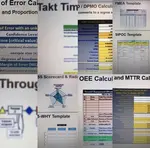
Six Sigma Templates, Tables, and Calculators. MTBF, MTTR, A3, EOQ, 5S, 5 WHY, DPMO, FMEA, SIPOC, RTY, DMAIC Contract, OEE, Value Stream Map, Pugh Matrix
Recent Articles
-
Process Capability Indices
Oct 18, 21 09:32 AM
Determing the process capability indices, Pp, Ppk, Cp, Cpk, Cpm -
Six Sigma Calculator, Statistics Tables, and Six Sigma Templates
Sep 14, 21 09:19 AM
Six Sigma Calculators, Statistics Tables, and Six Sigma Templates to make your job easier as a Six Sigma Project Manager -
Six Sigma Templates, Statistics Tables, and Six Sigma Calculators
Aug 16, 21 01:25 PM
Six Sigma Templates, Tables, and Calculators. MTBF, MTTR, A3, EOQ, 5S, 5 WHY, DPMO, FMEA, SIPOC, RTY, DMAIC Contract, OEE, Value Stream Map, Pugh Matrix -
Six Sigma, Six Sigma Training, Courses, Calculators, Certification
Aug 15, 21 10:27 PM
 One site with the most common Six Sigma material, videos, examples, calculators, courses, and certification.

Site Membership
LEARN MORE
Six Sigma
Templates, Tables & Calculators
Six Sigma Slides
Green Belt Program (1,000+ Slides)
Basic Statistics
Cost of Quality
SPC
Control Charts
Process Mapping
Capability Studies
MSA
SIPOC
Cause & Effect Matrix
FMEA
Multivariate Analysis
Central Limit Theorem
Confidence Intervals
Hypothesis Testing
Normality
T Tests
1-Way ANOVA
Chi-Square
Correlation
Regression
Control Plan
Kaizen
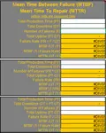
MTBF and MTTR
Project Pitfalls
Error Proofing
Z Scores
OEE
Takt Time
Line Balancing
Yield Metrics
Sampling Methods
Data Classification
Practice Exam
... and more