Covariance

Covariance measures the relationship of two continuous variables and how they move together above and below their means. It's used to determine the direction of the linear relationship of two continuous variable. The values can range from -infinity to +infinity.

A positive value indicates that two variables move in the same direction.
A negative value indicates movement in opposite directions.

Keep in mind, this is not the same as Coefficient of Variation which is taught in the module called Measures of Dispersion. Also, the data sets of x and y do not need to be checked for normality to get useful Covariance or Correlation values.

This technique is commonly used in the stock market to reduce risk while generating the same return on investment. A portfolio of stocks will often consist of those that reduce risk together and do not always move in the same direction.

However, Correlation is more informative and should be used when possible instead of Covariance.

Sample Covariance Formula

Population Covariance Formula

Simply substitute N in place of (n-1) in the above formula. Also the mean of x and y are represented by mu (the population) for x and y since the population is being evaluated instead of the sample.

While the Covariance indicates how well two variables move together, Correlation provides the strength of the variables and is a normalized version of Covariance. They both will always have the same sign: positive, negative, or 0.

Covariance is the numerator in the equation below therefore if the standard deviations of x and y are constant, as the Covariance increases, the Correlation also increases and approaches +1.0. Also, if the Covariance decreases, the Correlation decreases and approaches -1.0.

Correlation is a dimensionless value that will always be between -1.0 and +1.0, with 0 indicating the two variables move randomly from each other and are uncorrelated. Values closer to 0 (either negative or positive indicate weaker and weaker correlation.

As Covariance increases (also as Correlation values approach +1.0) this indicates a stronger and stronger positive relationship of the variables moving together. As Covariance decreases (also as correlation values approach -1.0) this indicates a stronger inverse relationship (see Example Three below).

Values near zero for both parameters equates to no relationship or correlation and therefore those inputs or combination of inputs are not related to the output. This is valuable to the Six Sigma team so this input can be ruled out (unless it has a impact as in a combination with another input).

The following formula illustrates the relationship of the two terms. The formula below applies for sample and population calculations.

Covariance using Excel

Finding Covariance for a sample or population using Excel is shown below.

Sample: covariance.S(array1, array2)

Population: covariance.P(array1, array2)

Create an array (one array per column) in Excel and the range of the array goes in the bracket. It does not matter which array is entered first in each of the formulas.

See the examples below that show various changes in data sets and the impact that those changes have on Covariance and Correlation values.

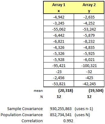
Example One

This example has 12 samples of highly erratic numbers but the Covariance is very strong as is the Correlation, both data sets move together.

The values for the Covariance appear to be very high, but how high is that? It is subjective. Therefore, using the Correlation in combination with Covariance helps to understand the degree of the relationship.

Example Two

In the example, all the same values are used as above but they are negative. Notice the Covariance values and Correlation value are the same as above. This illustrates that fact the the relationship may be just as strong regardless if the data set values are positive or negative.

There remains are very strong correlation between the input to the output. This is a valuable tool when a Six Sigma team is looking to control the the key input and understand to what degree it affects the output.

Example Three

In this example, the data is going in opposite directions and thus the Covariance is negative. See the chart at the bottom. Also, notice the Correlation is strongly negative at close to -1.0 so this also indicate an inverse relationship of x and y. As an input x increase by an amount, the output y is very likely to decrease by a similar amount.

Again, this is powerful insight for a Six Sigma team to have a strong understanding (whether good or bad) on which variable(s), to what extent, affect the output.