|

 content.")

Alpha and Beta Risks
Alpha Risk
Alpha risk (α) is the risk of incorrectly deciding to reject the null hypothesis, HO. If the chosen confidence level is 95%, then the alpha risk is 5% or 0.05.
For example, there is a 5% chance that a part has been determined defective when it actually is not. One has observed, or made a decision, that a difference exists but there really is none. Or when the data on a control chart indicates the process is out of control but in reality, the process is in control. Or the likelihood of detecting an effect when no effect is present.
Alpha risk is also called False Positive, Type I Error, or "Producers Risk".
Confidence Level = 1 - Alpha Risk = 1 - α
Alpha is called the significance level of a test. The level of significance is commonly between 1% or 10% but can be any value depending on your desired level of confidence or need to reduce Type I error. This type of risk can only occur when HO is rejected.
Selecting 5% signifies that there is a 5% chance that the observed variation is not actually the truth. The most common level for alpha risk is 5% but it varies by application and this value should be agreed upon with your BB/MBB.
In summary, it's the amount of risk you are willing to accept of making a Type I error.
If conducting a 2-sample T test and your conclusion is that the two means are different when they are actually not would represent Type I error:
EXAMPLES:
- A carbon monoxide alarm indicating a high-level alert but there is actually not a high level - this is a Type I error.
- The probability of scrapping good parts when there is not an actual defect. The "Producer" is taking a risk of losing money due to an incorrect decision, hence the analogy of why alpha-risk is also known as "Producer's Risk".
- The probability of convicting an innocent person.
Beta Risk
Beta risk (β) is the risk that the decision will be made that the part is not defective when it really is. In other words, when the decision is made that a difference does not exist when there actually is. Or when the data on a control chart indicates the process is in control but in reality, the process is out of control.
If the power desired is 90%, then the beta risk is 10%. There is a 10% chance that the decision will be made that the part is not defective when in reality it is defective.
Contrary to alpha risk, beta occurs when HO is not true (or is rejected).
Power = 1 - Beta risk = 1 - β
Beta risk is also called False Negative, Type II Error, or "Consumer's" Risk.
The Power is the probability of correctly rejecting the Null Hypothesis.
The Null Hypothesis is technically never proven true. It is "failed to reject" or "rejected".
"Failed
to reject" does not mean accept the null hypothesis since it is
established only to be proven false by testing the sample of data.
Guidelines: If the decision from the hypothesis test is looking for:
- Large effects or LOW risk set Beta = 15% (which is Power of 0.85)
- Medium effects, MEDIUM risk but not catastrophic, legal or safety related the set Beta = 10%
- Small effects, HIGH risk, legal, safety, or critical set beta from 5% to near 0%.
If conducting an F-test and your conclusion is that the variances are the same when they are actually not would represent a Type II error.
Typically, this value is set between 10-20%.
Same note of caution as for alpha risk, the assumption for beta risk should be agreed upon with your BB/MBB.
EXAMPLES:
The risk of passing parts that are actually defective. The "Consumer" is taking a risk of due to the Producer making an incorrect decision and putting these bad parts out for the Consumer (or customer) to use or purchase, hence the analogy of why beta-risk is also known as "Consumer's Risk".
The risk (or probability) of not convicting (releasing) someone that is actually not innocent.
Decision Matrix
Visual Aid One

Visual Aid Two
This matrix below is available for free for subscribers.

Sampling
The size of the sample must be consciously decided on by the Six Sigma Project Manager based on the allowable alpha and beta risks (statistical significance) and the magnitude of shift that you need to observe for a change of practical significance.
As the sample size increases, the estimate of the true population parameter gets stronger and can more reliably detect smaller differences.
The best way to reduce both types of error is to increase the sample size which is logical since you are getting closer to the population and the larger samples become more representative of
This seems logical, the closer you get to analyzing all the population, the more accurate your inferences will be about that population.
It is not possible to commit both Type 1 and Type II error simultaneously on the same hypothesis test.
More information about sampling can be found here.
Hypothesis Testing Steps
Click here for more details on hypothesis testing
- Define the Problem
- State the Objectives
- Establish the Hypothesis (left tailed, right tailed, or two-tailed)
- State the Null Hypothesis (HO)
- State the Alternative Hypothesis (HA)
- Select the appropriate statistical test
- State the alpha-risk level
- State the beta-risk level
- Establish the Effect Size
- Create Sampling Plan, determine sample size
- Gather samples
- Collect and record data
- Calculate the test statistic and/or determine the p-value
If p-value is < than alpha-risk, reject HO and accept the Alternative, HA
If p-value is > than alpha-risk, fail to reject the Null, HO
Try to re-run the test (if practical) to further confirm results. The next step is to take the statistical results and translate it to a practical solution.
It is also possible to determine the critical value of the test and use to calculated test statistic to determine the results. Either way, using the p-value approach or critical value provides the same result.
One Tail or Two Tail?
Hoo: Mean A = Mean B is a two-tailed hypothesis
Ho: Mean A < Mean B is a one-tail hypothesis
Ho: Mean A > Mean B is also a one-tail hypothesis
In a one-tail test, the enter rejection region is on one side of the distribution. In a two-tail test the rejection regions exist on both sides of the distribution, above and below the critical value.


More about Alpha and Beta Risks - Download
 |
Click here to purchase a 1000+ Six Sigma Training Slides includes topics covering hypothesis testing, risk and power. Other topics within Six Sigma are also available. |
Confidence INTERVAL vs. Confidence LEVEL
What is the difference between a Confidence Level and Confidence Interval?
The Confidence Level refers to the percentage of probability, or certainty, that the Confidence Interval would contain the true population parameter when you draw a random sample repeatedly.
Often results are shown for a “95% Confidence Interval” …. this means there is a 95% Confidence Level that the Confidence Interval contains the population parameter and 5% risk (alpha) of the Confidence Interval not containing the population parameter.
Test your knowledge with these Six Sigma certification questions
Return to Six-Sigma-Material Home Page
Recent Articles
-
Process Capability Indices
Oct 18, 21 09:32 AM
 Determing the process capability indices, Pp, Ppk, Cp, Cpk, Cpm
 -
Six Sigma Calculator, Statistics Tables, and Six Sigma Templates
Sep 14, 21 09:19 AM
 Six Sigma Calculators, Statistics Tables, and Six Sigma Templates to make your job easier as a Six Sigma Project Manager
 -
Six Sigma Templates, Statistics Tables, and Six Sigma Calculators
Aug 16, 21 01:25 PM
Six Sigma Templates, Tables, and Calculators. MTBF, MTTR, A3, EOQ, 5S, 5 WHY, DPMO, FMEA, SIPOC, RTY, DMAIC Contract, OEE, Value Stream Map, Pugh Matrix
Recent Articles
-
Process Capability Indices
Oct 18, 21 09:32 AM
Determing the process capability indices, Pp, Ppk, Cp, Cpk, Cpm -
Six Sigma Calculator, Statistics Tables, and Six Sigma Templates
Sep 14, 21 09:19 AM
Six Sigma Calculators, Statistics Tables, and Six Sigma Templates to make your job easier as a Six Sigma Project Manager -
Six Sigma Templates, Statistics Tables, and Six Sigma Calculators
Aug 16, 21 01:25 PM
Six Sigma Templates, Tables, and Calculators. MTBF, MTTR, A3, EOQ, 5S, 5 WHY, DPMO, FMEA, SIPOC, RTY, DMAIC Contract, OEE, Value Stream Map, Pugh Matrix -
Six Sigma, Six Sigma Training, Courses, Calculators, Certification
Aug 15, 21 10:27 PM
 One site with the most common Six Sigma material, videos, examples, calculators, courses, and certification.

Site Membership
LEARN MORE
Six Sigma
Templates, Tables & Calculators
Six Sigma Slides
Green Belt Program (1,000+ Slides)
Basic Statistics
Cost of Quality
SPC
Control Charts
Process Mapping
Capability Studies
MSA
SIPOC
Cause & Effect Matrix
FMEA
Multivariate Analysis
Central Limit Theorem
Confidence Intervals
Hypothesis Testing
Normality
T Tests
1-Way ANOVA
Chi-Square
Correlation
Regression
Control Plan
Kaizen
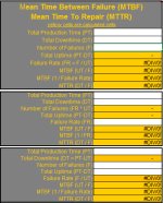
MTBF and MTTR
Project Pitfalls
Error Proofing
Z Scores
OEE
Takt Time
Line Balancing
Yield Metrics
Sampling Methods
Data Classification
Practice Exam
... and more