ShareFacebookXWhatsAppReddit

Design of Experiments (DOE)

Design of Experiments (DOE) is a study of the factors that the team has determined are the key process input variables (KPIV's) that are the source of the variation or have an influence on the mean of the output.

DOE are used by marketers, continuous improvement leaders, human resources, sales managers, engineers, and many others. When applied to a product or process the result can be increased quality performance, higher yields, lower variation of outputs, quicker development time, lower costs, and increased customer satisfaction.

It is a sequence of tests where the input factors are systematically changed according to a design matrix. The DOE study is first started by setting up an experiment with a specific number if runs with one of more factors (inputs) with each given two or more levels or settings. 

The DOE process has a significant advantage above trial and error methods. Yes, it may end up taking more time and resources but the result will most likely be more robust.

This initial time and effort up front can be costly (this is up to the team to decide how many experiments to conduct) and time consuming but the end result will be the maximizing the outputs shown above in bold. 

A DOE (or set of DOE's) will help develop a prediction equation for the process in terms of Y = f(X₁,X₂,X₃,X₄,....X_n).

GOAL:

1) Understand the influential variables and understand any interactions

2) Quantify the effect of the variables on the outputs

3) Determine the setting that optimize your response (which could be to minimize or maximize an value for an output "y")

Designing a DOE

The number of runs (treatments) depends on amount of resources that can be afforded...such as time and money and keep in mind, replications are ideal to help validate the results and help detect any fluke results. 

The power of efficiency in a DOE is within hidden replication. However, the may be instances with a block design is incomplete when it isn't possible to apply all treatments in every block. 

More treatments takes more time and money but offers the most information. It's a trade-off between the amount of Type I and II error you can afford to risk along with time and money. 

The more factors and levels you have, the more combinations are possible and thus adding more time and money to the project, unless you choose to take more risk and reduce the runs by using a fractional design. Of course, being able to adjust setting of more variables and playing more with factors is great, but it comes with a price. 

The guide below shows that the amount of 'levels' to the power of the number of 'factors' is the number of combinations of treatments for a full factorial design. 

For example, with two factors (inputs) each taking two levels, a factorial DOE will have four combinations. With two levels and two factors the DOE is termed a 2×2 factorial design. A memory tactic....Levels lie low and Factors fly high

A DOE with 3 levels and 4 factors is a 3×4 factorial design with 81 (3⁴ = 81) treatment combinations. It may not be practical or feasible to run a full factorial (all 81 combinations) so a fractional factorial design is done, where usually half of the combinations are omitted.

STEPS to conduct a DOE:

1. Define the objective for the DOE
2. Select the process variables (independent and dependent)
3. Determine DOE design - which depends on resources (time & money) and amount of Type I and II error you're willing to accept
4. Execute the design (randomization where possible)
5. Verify results (replicate the tests if practical to help verify results)
6. Interpret the results

The next step is to implement IMPROVEMENTS (that’s the goal….implementing improvements that matter)

Here are some characteristics of factorial experiments in general:

• A Response is the output and is the dependent variable
• Response = sum of process mean + variation about the mean
• Factors are independent variables
• Variation about the mean is sum of factors + interactions + unexplained residuals (or experimental error)
  

ANOVA is used to decompose the variation of the response to show the effect from each factor, interactions, and experimental error (or unexplained residual).

Statistical software will help manage the entire DOE.

1. Enter the factors
2. Set the levels (at least two for each factor)
3. Determine how many runs (full factorial, fractional factorial)
4. Run the experiment at each treatment level
5. Enter the response for each treatment level
6. Use statistical software to use ANOVA on the data
7. Continue to refine until prediction equation is obtained
8. IMPROVE the KPIV's
9. Last phase is CONTROL the KPIV's
   

Other methods of experimentation such as "trial and error" or "one factor at a time (OFAT)" are prone to waste, will provide less information and will not provide a prediction equation. These may seem easier to run and get results but the risk is a less robust solution and decisions made on a poor experiment.

These input factors behave to create an output, the team needs to make improvements in the IMPROVE phase that control the inputs. Controlling the input factors will provide the desired response.

The DOE will quantify the factor interactions and offer a prediction equation. ANOVA will help indicate which factors and combinations are statistically significant and which are not thus giving direction to the priority of improvements.

DOE Assumptions since ANOVA is used to analyze the data:

1. The residuals are independent
2. The residuals have equal variance
3. The residuals are normally distributed
4. All inputs (factors) are independent of one another
   

Most prediction equations will be linear and reliable when using only two levels. This saves time and money while obtaining a prediction equation.

Prediction equations are useful to analyze what-if scenarios. Many times data can not be collected at all levels and factors so a prediction equation can be used to estimate the output.

The input factors are x's and the response is Y-hat.

Full Factorial DOE

The following are characteristics of a Full Factorial DOE:

• Usually results is large number of tests. If the number of parameters is large then the number of test becomes significantly large (there are more and more interaction combinations and possibilities).
• Testing every combination of factor levels.
• Captures all interactions which of course is nice to have but this comes at a cost and time.

For instance, if there 9 factors and 3 levels for each factor that the team wants to test, then that is 3⁹ = 19,683 runs to determine all the interactions! 

3 * 3 Full Factorial DOE

Using the same vehicle throughout and maintaining all external variables as constant as possible a study is being created to find a prediction equation for the miles per gallon (MPG). There are 27 runs needed to bring out all the interactions (3³).

The team has determined that coefficient of friction of surface, ambient temperature, and tire pressure are three critical input factors (KPIV's) to study.

The goal isn't always to maximize MPG but to understand the impact on vehicle MPG based on these factors. The problem statement may be to improve the accuracy of MPG claims on this specific vehicle.

The table below summarizes the three levels chosen for each of the three factors.

How many trials are required if you want to run a Full Fractional DOE with 5 factors at 4 levels each?

ANSWER: 4⁵ = 1,024 trials (this could be impractical...thus look into the option below).

Fractional Factorial DOE

A Fractional Factorial experiment uses subset of combinations from a Full Factorial experiment. They are applicable when there are too many inputs to screen practically or cost or time would be excessive. 

This type of DOE involves less time than One-Factor at a Time (OFAT) and a Full Fractional Factorial but this choice will result in less data and some interactions will be confounded (or aliased). This means that the effect of the factor cannot be mathematically distinguished from the effect of another factor.  

Most processes are driven by main effects and lower order interactions so choose the higher order interactions for confounding. Lower confounding is found with higher resolution.

If a half fractional factorial experiment is determined to be most practical and economical where there are two levels and five factors then there will be a combination of 16 runs analyzed. Usually higher order interactions are omitted to focus on the main effects.

DOE jargon

One-Way Experiment: involves only one factor. 

Response (Y, KPOV): the process output linked to the customer CTQ. This is a dependent variable.

Factor (X, KPIV): uncontrolled or controlled variable whose influence is being studied. Also called independent variables.

Inference Space: operating range of factors under study

Factor Level: setting of a factor such as 1, -1, +, -, hi, low.

Treatment Combination (run): setting of all factors to obtain a response

Replicate: number of times a treatment combination is run (usually randomized). Replication is done to estimate the Pure Trial Error to the Experimental Error. Replication is very important to under confounding and interactions.

ANOVA: Analysis of Variance

Blocking Variable: Variable that the experimenter chooses to control but is not the treatment variable of interest.

Interaction: occurrence when the effects of one treatment vary according to the levels of treatment of the other effect.

Main effect: estimate of the effect of a factor that is independent from any of the other factors.

Collinear: variables that are linear combinations of one another. Two perfectly collinear variables with an exact linear relationship will have correlation of -1 or 1.

Confounding: variables that are not being controlled by the experimenter but can have an effect on the output of the treatment combination being studied. It describes the mixing of estimates of the effects from the factors and interactions. Two (or more) variables are confounded if effects of two or more factor aren't separable.

One of the most commons mistakes in a DOE is to confound the effects of the variable that someone wants to estimate with that of another factor. which often times happens from improper randomization. 

Latin Square: This design of DOE has three types of effects

Randomized Block: This design has two types of effects: Treatment effects and Block effects

Sensitivity: refers to the ability to identify significant treatment differences in the response variable.

Covariate: Factors that change in an experiment that were not planned to change.

Explaining DOE

This is a lengthy video but it slowly but clearly teaches the concepts and jargon and then jumps into an example at the end. The prelude to the example helps put all the pieces together before diving into an example.

Other Types of DOE's

Taguchi's Design

Taguchi's Design uses orthogonal arrays to estimate the main effects of many levels or even mixed levels. A selected and often limited group of combinations are investigated to estimate the main effects.

The goal is to find and develop a parameter that can improve a performance characteristic. It can be used to look for alternative materials or design methods that deliver equivalent or better performance.

The intent is to reduce the quality loss to society. Taguchi has the concept of loss function and assumes losses when a process doesn't meet a target value. The losses are from the variation of a process output. He states that losses rise quadratically as they move from the target value to the LSL/USL (may be one or the other or both).

Signal to Noise (S/N) ratios are used to improve the design. Ideally, the output from the design should not react to variation from the noise factors. 

Plackett-Burman

Plackett-Burman - two level fractional factorial design that analyzes only a few selected combinations to evaluate on main effects and no interactions.

Response Surface Methodology

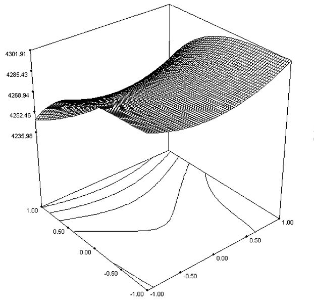
Response Surface Methodology (RSM) is used to study multiple factors although two are normally done.

RSM creates a map of the response from running a series of full factorial DOE's and comes up equations that describe how the factors affect the response.

RSM designs are used to refine processes after an experiment such as Plackett-Burman has identified the vital main effects. Then one can determine the settings of the factors to achieve of the desired response. 

Circumscribed Central Composite (CCC), Face Centered Composite (CCF), and Inscribed Central Composite (CCI) are designs that require 5 factor levels. As you can see in their names, these are all varieties of central composite designs. They are (and also Box-Behnken) RSM designs. 

RSM's may have a 3D response. Consider the following equation that came from an experiment:

y = 3.2 + 4.5x₁ + 5.2x₂ + 9x₂² + 8.2x₁x₂

The formula contains two slope components (4.5x₁ and 5.2x₂), and curve component (9x₂²) and a twist component (8.2x₁x₂)

Box-Behnken

Similar to the Face Centered Composite (CCF) in which it requires 3 factor levels

Considered a Response Surface Methodology Design

Circumscribed Central Composite (CCC)

Similar to Inscribed Central Composite (CCI) design which is also a higher order design and both require 5 factor levels.

Considered a Response Surface Methodology Design

Alpha, α, = [2^k]^1/4 where k = number of factors

Alpha is the distance of each axial point (star point) from the center in a central composite design. A value <1 puts the axial points in the cube; a value =1 puts them on the faces of the cube; and a value >1 puts them outside the cube.

Return to the IMPROVE phase

Get access to all the material within this site

Search active Six Sigma job openings

Return to Six-Sigma-Material Home Page

Recent Articles

• 
• 
• 

1. Process Capability Indices

   Oct 18, 21 09:32 AM

   
   Determing the process capability indices, Pp, Ppk, Cp, Cpk, Cpm

   Read More

2. Six Sigma Calculator, Statistics Tables, and Six Sigma Templates

   Sep 14, 21 09:19 AM

   
   Six Sigma Calculators, Statistics Tables, and Six Sigma Templates to make your job easier as a Six Sigma Project Manager

   Read More

3. Six Sigma Templates, Statistics Tables, and Six Sigma Calculators

   Aug 16, 21 01:25 PM

   
   Six Sigma Templates, Tables, and Calculators. MTBF, MTTR, A3, EOQ, 5S, 5 WHY, DPMO, FMEA, SIPOC, RTY, DMAIC Contract, OEE, Value Stream Map, Pugh Matrix

   Read More